Contents
1. Beam Pattern
2. L-band Pointing Accuracy for 40-m TNRT
3. Amplitude Calibration with Noise Source Injection
4. Aperture Efficiency with its Dependence along Elevation
5. RFI Bird's-eye View Distribution at TNRO Site
6. Skyline Bird's-eye View Map
7. Linearity Net in the L-band System
8. Limitation of Integration Time at Each Observation Scanning
10. Sensitivity
11. Observation Scanning Modes
12. References
Beam pattern of the 40-m TNRT in L-band was measured in 9-11 August 2023 by observing a strong continuum source M87 (3C274, Virgo A) that is listed in the catalog of compact and flux well-known calibrators by Perley, R. A. & Butler, B. J. (2017, ApJS, 230, 7). Although M87 is the well-known source showing a diffuse structure with extended radio lobes across the angular size of around 14 arcmin, the compact brightest core in the center that contains the one-sided jet showed the angular size smaller than 5 arcmin, which could be assumed as a moderate point-like source for a single-dish radio telescope beam in L-band. The observations measuring the TNRT L-band beam pattern were conducted via 1-sec integrating in frequency range of 1.63-1.67 GHz for the vertical linear polarization at each location on the raster scan grid of 250 arcsec. In these observations, OFF source data were obtained in each date at each different EL of 10, 15, 20, 25, 30, 40, 50, and 60 deg. Total-power in 1.63-1.67 GHz was converted into be an antenna temperature Ta* [K] via injecting the Noise-Source at each grid scan (see section "Amplitude Calibration with Noise Source Injection" for the Noise-Source temperature and the conversion procedure in detail).
As a result, the beam pattern is represented in mapping area of 8,000 × 8,000 arcsec2, as shown in figure 1-1 (Left: 2-dimension, Right: 3-dimension).
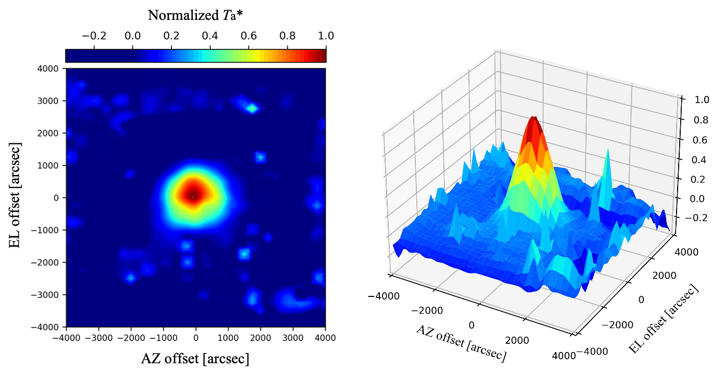
Quantitatively, the beam size was estimated by 2-dimensional Gaussian fitting expressed in the following equation:
P (∆AZ, ∆EL) = a * exp−4 ln(2)𝜇az − ∆AZHPBWaz2−4 ln(2)𝜇el − ∆ELHPBWel2
where a is the measured brightest antenna temperature, 𝜇az and 𝜇el are pointing offsets in the AZ and EL directions, and HPBWaz and HPBWel are the half-power beam width in the AZ and EL directions, respectively. The best fit parameters are shown in Table 1-1.
Based on this estimation, the beam pattern of the TNRT L-band is slightly distorted by being 1.14 times elongated in the AZ direction larger than one in the EL direction.
| Type |
Mean ± Standard deviation (arcsec) |
|---|---|
| HPBWaz | 1,462 ± 47 |
| HPBWel | 1,287 ± 41 |
| 𝜇az | −26 ± 20 |
| 𝜇el | +68 ± 17 |
2. L-band Pointing Accuracy for 40-m TNRT
• Results
L-band pointing accuracies of TNRT are 176 and 96 (arcsec) in Az and El directions, respectively (see Table 2-1 and Fig. 2-1). The pointing accuracies in Az and El directions correspond to 12% and 7% of TNRT beam size, respectively. To determine Az and El offsets, we fitted cross scan data with a Gaussian function. As a result, mean values of Full Width at Half Maximum (FWHM) in Az and El are consistent with TNRT beam sizes in Az and El, respectively, within 1.5-𝜎. It means that pointing calibrators observed are compact.
| Type |
Mean ± Standard deviation (arcsec) |
Nscans |
|---|---|---|
| Az offset | 88 ± 176 | 544 |
| El offset | 8 ± 96 | 544 |
| Az FWHM | 1284 ± 105 | 544 |
| El FWHM | 1286 ± 102 | 544 |
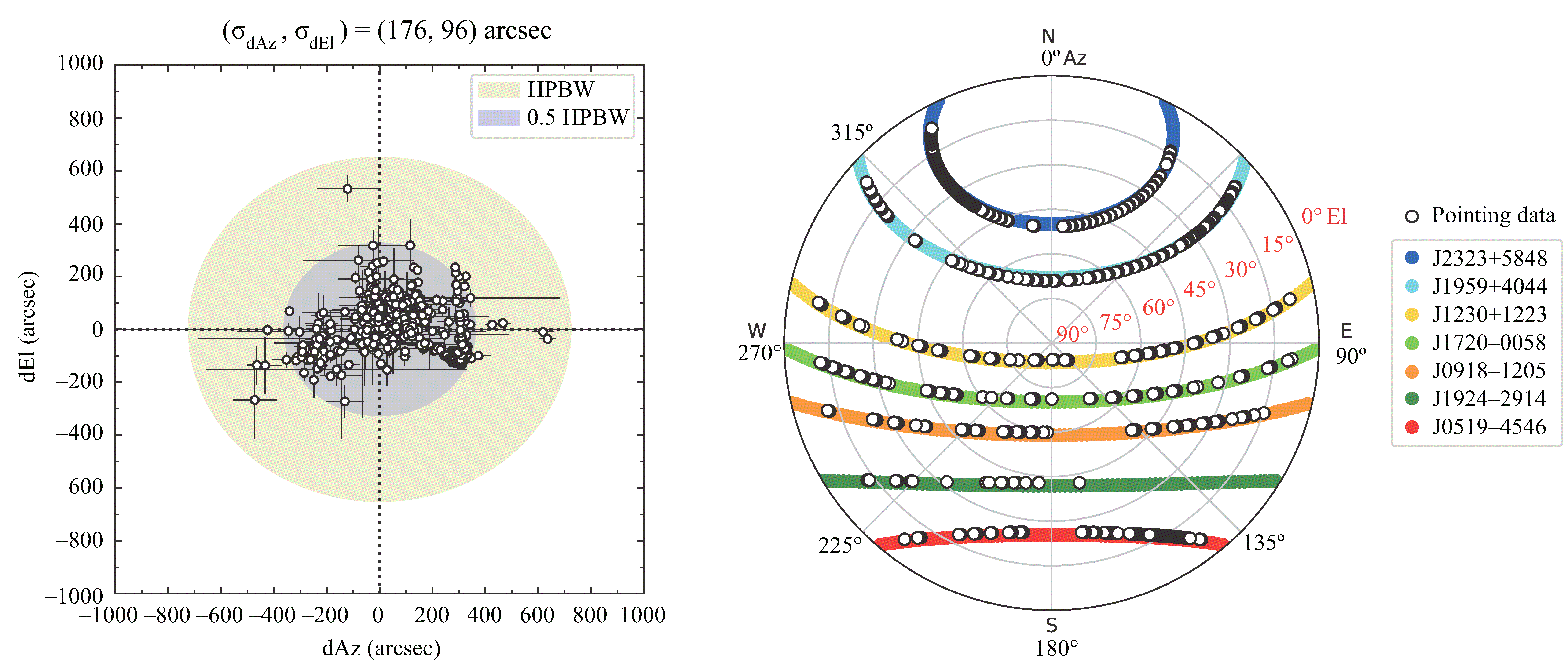
Figure 2-1: (Left) L-band TNRT pointing results, Az offset (dAz) and El offset (dEl) values, are shown. The number of data points is 544. Standard deviations of (dAz, dEl) are 176 and 96 (arcsec), respectively. Yellow and blue ellipses indicate the Half Power Beam Width (HPBW) and 50% HPBW of TNRT, respectively. (Right) 544 data points (white circles) used in (Left) are plotted on the polar projection of the sky in horizontal coordinates. Note that East is shown in right side, rather than left. We observed seven continuum sources listed by Perley & Butler (2017) and the VLBA Calibrator Search Tool. Individual trajectories of the seven sources are shown by different colors.
• Pointing model
Regarding TNRT pointing model, we referred to de Vicente & Barcia (2007) which introduced a pointing model for Nasmyth telescope. Using the model, Az and El offsets are described as
de Vicente & Barcia (2007) explained physical meanings of individual pointing coefficients/parameters (see Table 2-2).
| Parameter | Physical meaning |
|---|---|
| P1 | Azimuth encoder offset. If positive the antenna always point towards larger azimuth values. This term also includes positioning errors for receivers in the Nasmyth focus. |
| P2 | Collimation error. It includes positioning errors for Nasmyth mirrors. |
| P3 | Lack of orthogonality between the azimuth and elevation axes. If positive both axis form an angle smaller than 90º. This term also includes positioning errors for receivers in the Nasmyth focus. |
| P4 | Tilt of azimuth axis along a E-W direction. If positive the axis is tilted towards the East. |
| P5 | Tilt of azimuth axis along a N-S direction. If positive the axis is tilted towards the South. |
| P4 | Tilt of azimuth axis along a E-W direction and N-S direction. Since it is a combination, the sign does not inform about the direction of the axis tilt. |
| P5 | Tilt of azimuth axis along a N-S direction and E-W direction. Since it is a combination, the sign does not inform about the direction of the axis tilt. |
| P7 | Elevation encoder offset. If positive the antenna always points towards higher elevations. It also includes positioning errors for Nasmyth mirrors. |
| P8 | Gravitational effects. It also includes positioning errors for receivers in the Nasmyth focus. |
| P9 | Gravitational effects. It also includes positioning errors for receivers in the Nasmyth focus. |
• Pointing procedures
Firstly, we determined only large constant offsets (i.e., P1 and P7) by observing a pointing calibrator J1959+4044 (Cyg-A) listed by Perley & Butler (2017). During pointing observations, we conducted cross scans in Az and El directions with each scan length of 10,560 (arcsec). 112 data points with each integration time of 0.536 (sec) were obtained along each Az or El scan, which gives a spatial spacing between individual data points of 94 (arcsec). Also, we recorded radio frequency between 1630 and 1670 MHz during the pointing observations. The frequency range is relatively Radio Frequency Interference (RFI) quiet in the TNRT L-band.
Secondly, we observed seven pointing calibrators covering a wide range of Az and El (see Fig. 2-1) so that we can determine all pointing parameters (P1, P2, P3, P5, P7, P8, P9).
Lastly, we observed the same calibrators with the pointing parameters determined above so that we can evaluate the pointing accuracy of TNRT (see Table 2-1).
• Discussions
We failed pointing observations in some (Az, El) coordinates although we observed bright continuum sources based on Perley & Butler (2017) and the VLBA Calibrator Search Tool. Comparison between Figure 2-1 (success results) and Figure 2-2 (failure results) indicates that the pointing failure is related to high system noise temperature due to strong RFI. The worst success rate (17%) was obtained for J1924-2914 which is the faintest source (~10 Jy) among the seven pointing calibrators.
The current pointing accuracy is smaller than 12% of the TNRT beam size, which guarantees scientific observations. However, the pointing accuracy of Az direction is 1.8 times worse than that of El direction. Also, the mean value of Az offset results deviates from zero value (88+/-176 arcsec) compared to that of El offset results (8+/-96 arcsec). We are still investigating how to improve the pointing accuracy of Az direction as an antenna commissioning item. To further improve the current pointing accuracy of TNRT, we will conduct antenna commissioning observations in parallel with scientific observations in this semester (Cycle 0; Resident Shared Risk Observing).
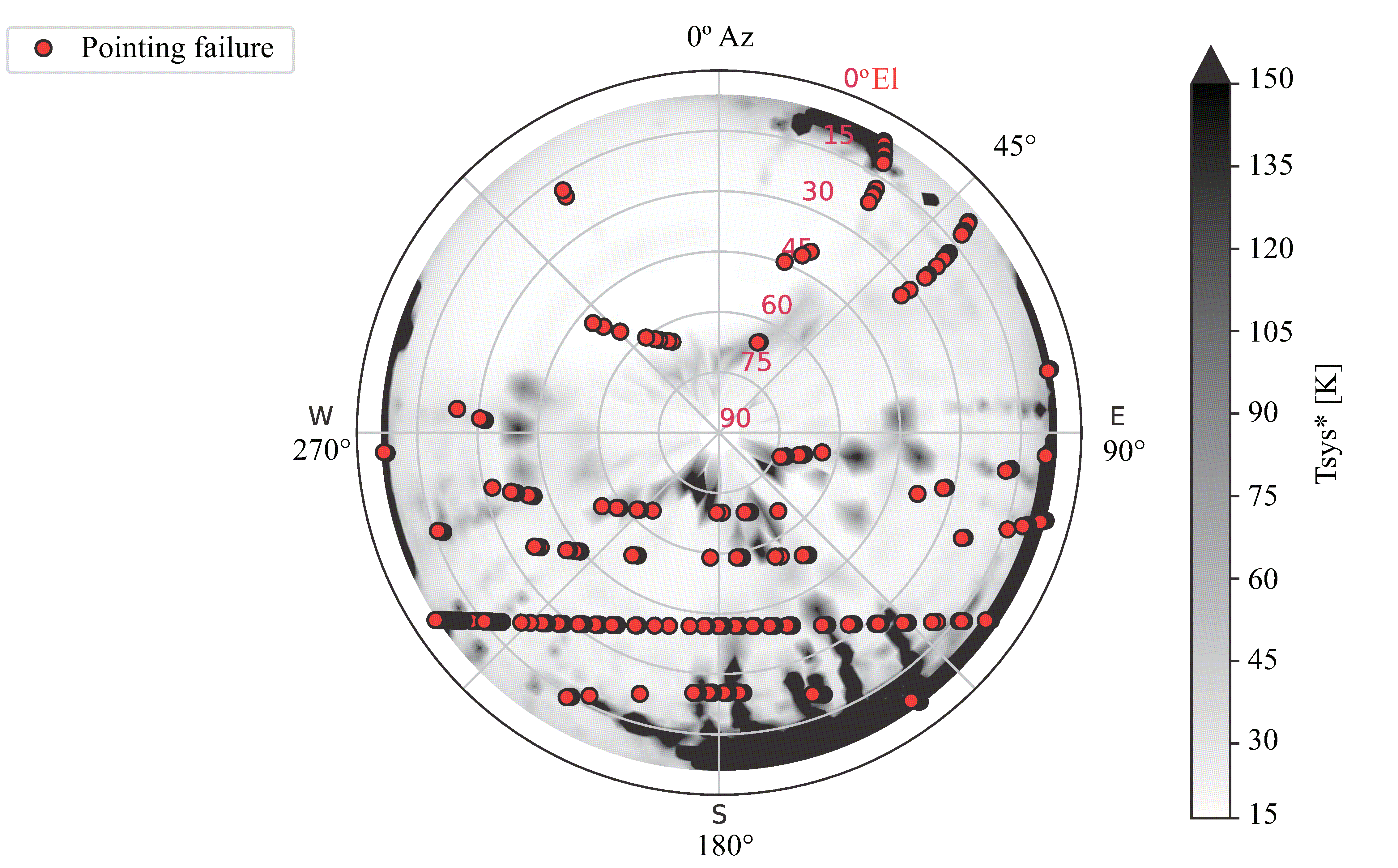
Figure 2-2: Red circles showing pointing failure results are superimposed on the polar projection of the sky in horizontal coordinates. The background showing system noise temperature (Tsys* in Kelvin) was obtained by TNRT skyline observations (see the section ''Skyline Bird's-eye View Map'' for details).
3. Amplitude Calibration with Noise Source Injection
Conversion of a total-power into an antenna temperature for the amplitude calibration in the TNRT L-band system is achieved by injecting a Noise-Source (NS). The injection of this NS consists of each sub-scan with this percentage: NS-ON 0.25% and NS-OFF 99.75%. So, for example, each accumulation period of each subscan data of 1 sec gives us NS-ON 0.0025 sec (to be used for calibration) & NS-OFF 0.9975 sec (to be used for integration to detect a target astronomical source), although both of them shows the same time stamp.
A system noise temperature Tsys* can be calculated by injecting a NS as follows:
Tsys* =TnsPsky+nsPsky − 1 exp(𝜏)
where Tns is a temperature of NS [K], Psky+ns and Psky are observed power with and without injecting NS, and 𝜏 is an optical depth. The essential factor Tns in the TNRT L-band was practically determined via temporary attaching an absorber on the horn that enables us to observe a black body emission with a temperature equivalent to an ambient temperature, with secZ way according to the following equations:
Tns = (Trx + Tamb) PR+nsPR − 1
ln (Tsys* + Tamb) = 𝜏0 secZ + ln (Trx + Tamb + Tbg)
where Trx, Tamb, Tbg are temperatures of a receiver, ambient environment, and background, respectively, and PR+ns and PR are observed power in cases of covering the horn by the absorber with and without injecting the NS, respectively. 𝜏0 is an optical depth at zenith.
As a result, Tns was determined to be 30.9 ± 1.1 [K]. while 𝜏0 was estimated to be 0.0098 ± 0.0004 as a bi-product.
Verification that this Tns works well was completed by comparing Tsys* measured by injecting the NS to the ones by R-Sky with the absorber. Along the secZ axis, Tsys∗ consistently ranged between 15 and 30 K within 10% errors using either of the methods, as shown in figure 3-1 on two different tracks at AZ = 330 and 294 deg (NS: red, R-Sky: blue). The best Tsys∗ of around 15 K signifies that this L-band receiver developed in collaboration with MPIfR (Gundolf Wieching et al.) is one of the best low-noise sensitive receivers in the world.
At the end, an antenna temperature Ta* can be calculated as follows:
Ta* = Tsys* PonPoff − 1
where Pon and Poff are observed power of ON astronomical source and OFF source (Sky), respectively.
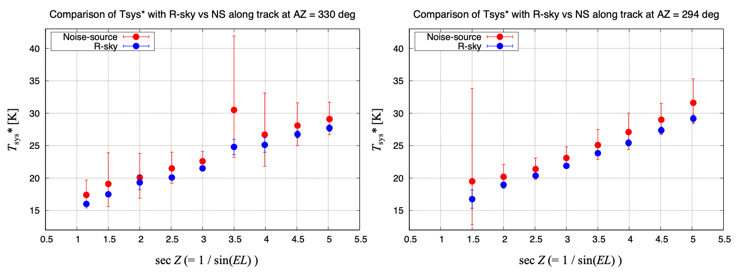
Figure 3-1: System noise temperature Tsys* versus secZ. Tsys* measured with injecting the noise-source and R-sky methods are shown by red and blue circle symbols, respectively, on two different tracks of AZ = 330 (left) and 294 deg (right).
4. Aperture Efficiency with its Dependence along Elevation
The aperture efficiency of the TNRT L-band system, in which the receiver is installed at the prime focus, was measured in July-August 2023 by observing strong and moderate / complete compact continuum calibrators whose flux densities with its stability in L-band are well-known as listed in Perley, R. A. & Butler, B. J. (2017, ApJS, 230, 7): we selected three sources M87 (3C274, Virgo A), Hydra A (3C218), and Hercules A (3C348). The observations were conducted in a frequency range of 1.63-1.67 GHz for the vertical linear polarization. These calibrators cover the wide range of the elevation direction, resulting in determining dependence of the aperture efficiency along elevation. The best fit result of the elevation dependence 𝜂A(EL) with a cubic function is as follows:
𝜂A(EL) = 1.13 × 10⁻⁶ EL3 −1.93 × 10⁻⁴ EL2 + 1.01 × 10⁻² EL + 0.365
and as shown in figure 4-1. The aperture efficiencies are achieved 50-53% with its stability in elevation higher than +20 deg, even while it keeps still beyond 40% in EL range of +4 to +20 deg.

Figure 4-1: Aperture efficiency of the TNRT L-band measured in 1.63-1.67 GHz for vertical linear polarization with its dependence along elevation. The red curve line presents the best fit on the observation data by a cubic function: 𝜂A(EL) = 1.13 × 10⁻⁶ EL3 −1.93 × 10⁻⁴ EL2 + 1.01 × 10⁻² EL + 0.365.
5. RFI Bird's-eye View Distribution at TNRO Site
To mitigate especially strong RFI impacts on the TNRT L-band system at the telescope site, a 90 cm parabolic reflector antenna (Rohde & Schwarz AC008 with HL024A1) was temporary installed at the top of the GNSS tower, which is located 40 m away from the TNRT in the North-East direction, as shown in figure 5-1. It enabled us to watch the same sky adaptable to the directions for the TNRT. The 1st trial of this RFI investigation was completed in March 2023. The observation data were recorded by using Keysight Fieldfox N9918B Spectrum analyzer used in the frequency range of 1-2 GHz with 100 kHz resolution bandwidth as both the max hold and averaged over 30 sec integration. These data were obtained at each 3 deg steps both in AZ and EL directions, resulting in the 1st release of a RFI bird's-eye view map at the telescope site in L-band, as shown in figure 5-2 (right).
This map constructed with total-power averaged over 30 sec and summed in 1-2 GHz frequency range presents that the power rises up to around 5 dB everywhere except for areas of EL higher than 45 deg and a part of the North-West direction. However, in the South-East direction at EL lower than 15 deg, we would like to emphasize that the super-strong RFI monster obstructs any observations due to super saturation of the L-band system, which might break the L-band receiver itself, in particular for the AZ range of 130-170 deg with rising the total-power up around 15 dB. Based on detailed investigations with spectra, e.g., figure 5-2 (left), a major contributor of those RFI monsters corresponds to a strong radio signal in 1.805-1.845 GHz, which could be caused by mobile base stations surrounding the telescope site.
In this CfP cycle, we have a plan to overcome this issue by avoiding those dangerous RFI monsters zones via implementing a dynamic scheduling with other target sources and/or flagging at post-processing. In forthcoming cycles of TNRT CfP, this issue will be solved in a forthcoming modification by producing high/low-pass bandpass filters that will be attached at just before the 1st low-noise amplifier (LNA) in the L-band receiver box, developed in collaboration with Max Planck Institute for Radio Astronomy (MPIfR). This will mitigate strong RFI impacts at the telescope site, which causes the saturation of total-power level of the L-band system, via drastic cutting-off those RFI outside of the effective bandwidths (1.0-1.8 GHz).
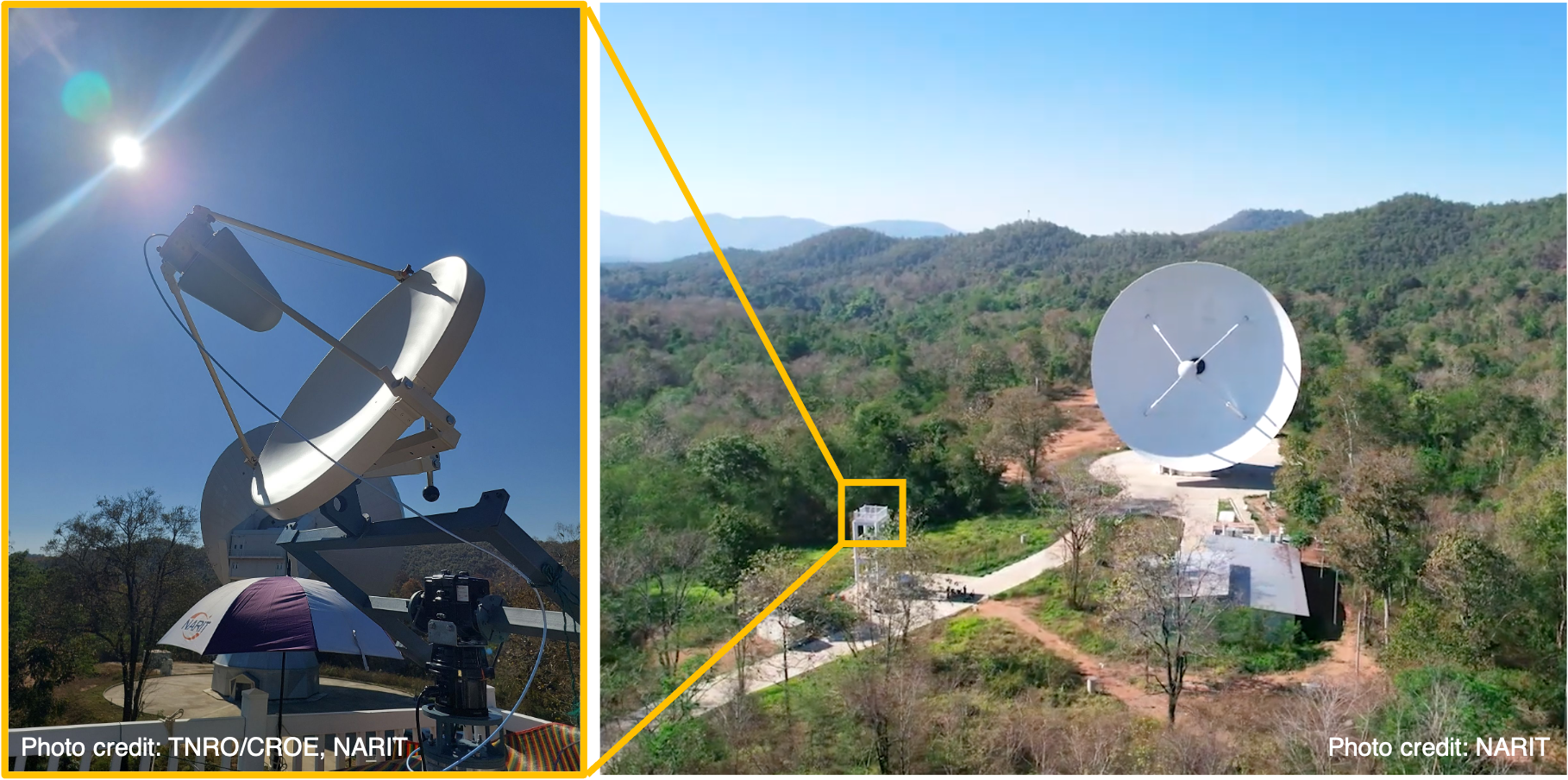
Figure 5-1: The 90 cm parabolic reflector antenna (left) installed at the top of the GNSS tower, which is located 40 m away from the TNRT in the North-East direction (right).
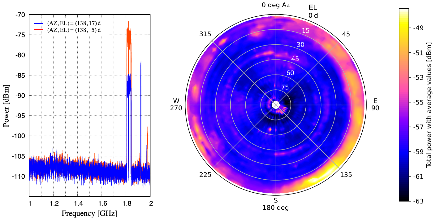
Figure 5-2: (Right) RFI bird's-eye view map observed with the 90 cm parabolic reflector antenna. Color code represents a total-power averaged over 30 sec and summed in 1-2 GHz frequency range in the unit of dBm (see the color scale in the right-hand side bar). (Left) An example of averaged spectra observed at (AZ, EL) = (138, 17) and (138, 5) deg shown by blue and red solid lines, respectively.
6. Skyline Bird's-eye View Map
For more in practically observations with the 40-m TNRT in the usable frequency range of this CfP cycle 1.63-1.67 GHz for the vertical linear polarization, skyline bird's-eye view maps observed with the 40-m TNRT itself are released as well, as shown in figure 6-1. These maps clarify even weaker but still impacting obstacles on the telescope. These observations were completed in February-April 2023 covering the whole sky coverage of AZ = 0-360 deg and EL = 6-85 deg with 2 or 5 deg angle steps. The data were integrated in 1.63-1.67 GHz usable bandwidth over 0.5 sec at each position for the vertical linear polarization, and converted from a total-power into a system noise temperature [K] with the Noise-source injecting method.
Figure 6-1 shows the skyline bird's-eye view maps in two different color code scales. Based on the left-panel in the Tsys* scale of 15-1,000 K, such strong RFI monster emissions at Tsys* higher than 1,000 K were confirmed to be consistent with the 90-cm RFI bird's-eye view map, but a bit more elongated to the positive AZ direction beyond +180 deg. Besides, this skyline map clarified another strong RFI area in a part of the North-East direction in EL lower than 10 deg with Tsys* beyond 1,000 K. On the other hand, the right-panel closing it up in the Tsys* scale of 15-300 K presented other dangerous zones to avoid: weird straight lines coming from the SE strong RFI monster zones even at EL higher than 30 deg and some hot spots in the East-West direction. Simultaneously, the right-panel bird's-eye view map clarified clear transparent zones observable with the best sensitivities of Tsys* = 15-30 K in the North-West direction with AZ = 280-360 deg, even in EL lower than 10 deg. Even with moderate Tsys* of around 2 times worse than the best, the areas shown by light-blue color code (between blue and cyan) spreading like radial pattern that covers all the sky except for the aforementioned areas/zones are acceptable for practical scientific observations. In the case of observing applicant's target sources across these moderate Tsys* areas, we recommend the applicants to consider taking into account around 2 times worse Tsys* for calculating the sensitivities required to achieve applicant's science goals.
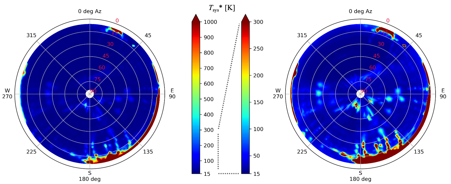
Figure 6-1: Skyline bird's-eye view maps observed with the 40-m TNRT L-band in 1.63-1.67 GHz for vertical linear polarization. Color code represents Tsys* [K] in the range of Tsys* 15 - 1,000 K (left) and 15 - 300 K (right), respectively (see the color scale at each side bar). Tsys* beyond the maximum value both in each plot is unified to be shown by deep red code.
7. Linearity Net in the L-band System
The linearity with its dynamic range net in the current TNRT L-band system was measured in Febuary-March 2023. This investigation was completed by observing in RFI quiescent / moderate blank sky areas, e.g., (AZ, EL) = (315,10), (315, 60) deg. The observations were achieved by controlling the Digital Step Attenuator (DSA: at being between 3rd and 4th amplifier in the L-band receiver box) from +30 dB (maximum) to +20 dB with 1 dB steps at each area and by measuring each output power as being integrated in 1.63-1.67 GHz for the vertical linear polarization.
Figure 7-1 presents the results of linearity investigations net in the current TNRT L-band system this time measured at position of (AZ, EL) = (315, 10) and (315, 60), respectively, both in which show the dynamic range ensuring the linearity up to 5 dB. In the viewpoint of injecting the Noise-source, reluctantly but it is acceptable because (Pns+sky − Psky) of 3-5 dB corresponds to Tsys* = 15−30 K. However, in the viewpoint of observing very strong continuum sources, note here that there is a practical restriction with flux densities of astronomical targets. Assumed that Tsys* = 20 K and the aperture efficiency = 50%, (Pon − Psky) of 5 dB corresponds to around 190 Jy. In the case of observing continuum sources showing its flux densities stronger than 190 Jy, the total-power will reach the saturation level and reliability of the absolute flux density might be decreased. In the case of proposing any observations for continuum target sources in this CfP cycle, we thus recommend to consider flux densities of applicant's target sources less than 190 Jy. On the other hand, there are no limitations at all for observing line emissions, e.g., masers, in this viewpoint of the dynamic range of the linearity.
This restriction will be fixed in the forthcoming modification by producing high/low-pass bandpass filters that will be attached at just before the 1st LNA in the L-band receiver box, developed in collaboration with MPIfR. This will mitigate strong RFI impacts at the telescope site, which causes the saturation of total-power level of the L-band system, via drastic cutting-off those RFI outside of the effective bandwidths (1.0-1.8 GHz).

Figure 7-1: Results of linearity investigations net in the current TNRT L-band system measured in 1.63-1.67 GHz for vertical linear polarization at position of (AZ, EL) = (Left) (315, 10) deg, and (Right) (315, 60) deg. This investigation was completed in a dynamic range of total-power 10 dB. The dashed line in each panel shows the case of achieving perfect linearity in this 10 dB total-power range.
8. Limitation of Integration Time at Each Observation Scanning
To clarify a practical limitation of integration times at each observation scanning without an ON-OFF switching method on the nearby sky in the current TNRT L-band system, the relation between reducing a standard deviation (1-sigma) of noise level and increasing integration times was investigated in April-May 2023 for 1.63-1.67 GHz frequency range usable in this CfP cycle. This investigation was completed at multiple positions of (AZ, EL) including the best transparent and the moderate Tsys* zones, respectively. In these observations, multiple set-ups for frequency channel resolution: 488, 244, 122, 61, 30, 15, 8, 4, and 2 kHz, were applied to verify the dependence according to the frequency resolutions. Besides, at post-processing stage, the data were analyzed in each different frequency range from 1.63 to 1.67 GHz with 0.01 GHz steps, respectively.
As a result, frequency channel resolutions better than 4 kHz are recommended to achieve the longest integration time at each observation scanning, even in observations for continuum target sources. As shown in figure 8-1, improvement of 1-sigma rms noise level according to increment of integration times without ON-OFF switching is limited up to 10 sec in particular in the frequency range of 1.63-1.64 GHz, while the limitation is softened to be longer than 100 sec in 1.65-1.67 GHz. The aforementioned restriction in 1.63-1.64 GHz could be caused by a weak spurious standing at around 1.637 GHz and this spurious seems like to be unstable in around a 10-sec period. We have a plan to execute an ON-OFF switching method on the nearby sky every 10 sec cycle to overcome this limitation in this CfP cycle.
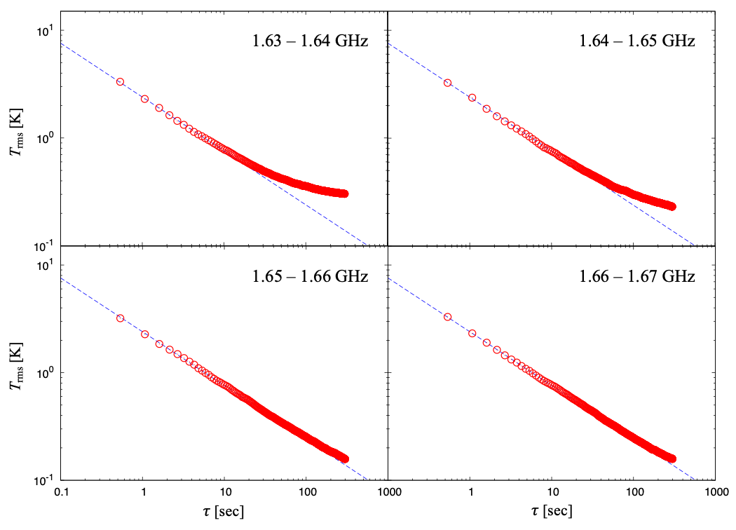
Figure 8-1: Integration times limited without ON-OFF switching method in the current TNRT L-band system measured with vertical linear polarization in each different frequency range from 1.63 to 1.67 GHz with 0.01 GHz steps, respectively. The vertical and horizontal axis corresponds to 1-sigma rms noise level [K] in a spectral channel with the frequency channel resolution of 3.82 kHz and net integration time 𝜏 [sec], respectively. The blue dashed line shows the case according to improvement by the inverse of square root of 𝜏.
Any Doppler tracking system in real time is not implemented in the current TNRT L-band system. The Doppler correction is thus performed at a post-processing calibration stage. This calibration works by calculating a velocity due to a Doppler effect at observatory, TNRO, on observing time corrected toward a target source direction in the Local Standard of Rest (LSR) frame with a developed python code.
Based on practical measured values of Tsys* = 15-30 K and typical aperture efficiency 𝜂A of 50% that is equivalent to degrees per flux unit (DPFU) of 0.23 K/Jy, and given the 8-bit sampling executed in the L-band receiver box for A/D conversion, a system equivalent flux density (SEFD) in the unit of Jansky of the current TNRT L-band system can be typically estimated by using the equation below:
SEFD = (2 k Tsys*)1026𝜂bit 𝜂A 𝝅D22
into be 66-132 Jy, where k is the Boltzmann constant, 𝜂bit is a coefficient to calibrate the quantization loss (≈ 1 in the case of 8-bit sampling), and D is the diameter of a telescope in the unit of meter.
As a result, an rms noise level 𝜎rms in the case of observing with the integration time 𝝉 of 10 min for a continuum and maser line emissions, respectively, can be typically calculated by using the equation below:
𝜎rms = SEFD(∆𝝂 𝝉)1/2
into be
Continuum case: 𝜎rms = 0.43 SEFD66 Jy40 MHz∆𝝂1/210 min𝝉1/2 mJy
Maser line case: 𝜎rms = 62 SEFD66 Jy1.9 kHz∆𝝂1/210 min𝝉1/2 mJy
where ∆𝝂 is a usable bandwidth assumed here to be 40 MHz and 1.9 kHz for continuum and maser emissions, respectively. We recommend applicants to fix the aforementioned usable bandwidth in your calculations, however an integration time is flexible depending on applicant's scientific requirement. Applicants are requested to consider a detection limit at least of 3 𝜎rms or higher to detect the target sources and to achieve applicant's scientific goals.
11. Observation Scanning Modes
In this CfP cycle, three observing scanning modes below are available:
[Single pointing] this mode is generally used for operations toward point (or point-like) target sources, unless other observing modes are requested.
[Cross scan] (e.g., figure 11-1 a) if applicants are concerned for less positional accuracies of the target source coordinates, this mode is recommended.
[Raster scan] (e.g., figure 11-1 b) this mode is recommended for a mapping observation toward diffuse target sources. The number of grids and a separation among each grid can be set flexibly. Typical overhead in the raster scan mode is around 30% of the total scanning time.
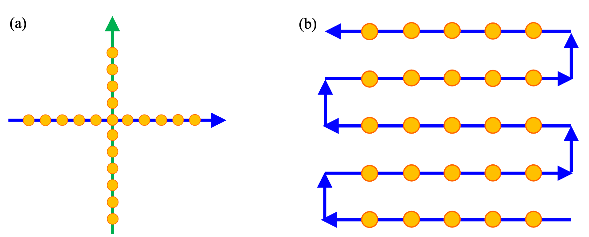
Figure 11-1: Schematic views of (a) cross scan mode, and (b) raster scan mode (an example in the case of 5 × 5 grid raster scan).
- de Vicente, P. & Barcia, A. 2007, Informe Técnio IT-OAN 2007-26
- Perley, R. A. & Butler, B. J. 2017, ApJS, 230, 7
- VLBA Calibrator Search Tool