Contents
2. The main and satellite lines of OH masers
3. References
For H I (1.42 GHz) commissioning of 40-m TNRT, we observed an H I standard region S8 (l = 207 deg, b = –15 deg) listed in Williams, D. R. W. 1973 with 40-m TNRT on October, 2024. The frequency resolution of the observation was 1.9 kHz corresponding to a velocity resolution of 0.4 km s-1. The on source time was 30 sec. Dual linear polarization (Vertical & Horizontal) data were recorded.
TNRT output file (MBFITS; Multi-Beam FITS; Muders, et al. 2006) was analyzed by standard procedures as
- Sky subtraction
- The determination of Tsys* (opacity corrected system noise temperature)
- The determination of Ta* (opacity corrected antenna temperature)
- Unit conversion from Kelvin (K) to Jansky (Jy)
- Conversion to the brightness temperature (TB; Kelvin)
- The correction of the Doppler effect.
The detail of the TNRT data reduction is summarized in the "Data reduction" section of this web page. Since 40-m TNRT observation at L-band cannot support the frequency switching, we employed the position switching for step 1. Even though we observed relatively H I free region at (l = 63 deg, b = +78 deg) for obtaining the sky data, H I emission is detected anywhere in the Milky Way and thus the sky data may degrade the absolute value of brightness temperature in the target data. For step 5, we referred to "Useful equations for radio astronomy"
We compared S8's spectrum obtained with 40-m TNRT with those obtained with other telescopes (see Figure 1-1; Table 1-2). Given a typical amplitude calibration error of single-dish data (~10 %) and different velocity resolutions, individual spectra are consistent with each other. However, the amplitude value of TNRT result may be underestimated due to the sky data which have small amount of H I emission. Although further investigation of H I observation with 40-m TNRT will be required, we accept H I observation with 40-m TNRT in this semester. Also, H I mapping observation with raster scanning is also accepted in this semester even though the H I mapping is under science commissioning
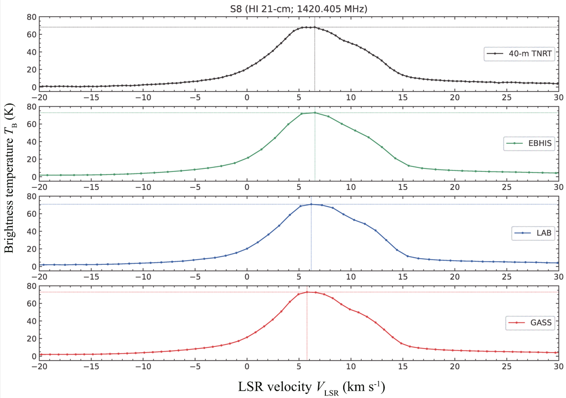
| Telescope |
Maximum brightness temperature, TB, max [K] |
VLSR at TB, max [km s-1] |
Velocity resolution [km s-1] |
|---|---|---|---|
| 40-m TNRT | 67.9 | 6.5 | 0.4 |
| Effelsberg 100-m | 72.9 | 6.5 | 1.3 |
| Dwingeloo 25-m | 70.7 | 6.2 | 1.0 |
| Parkes 64-m | 72.9 | 5.8 | 0.8 |
2. The main and satellite lines of OH masers
Example spectra of the main and satellite lines of OH masers obtained with 40-m TNRT are shown in Figures 2-1 and 2-2. We confirmed only small fluctuations in the spectra of VY CMa for about 70 days (Figure 2-2 (bottom)), which are lower than 8 %, 13 % and 5 % for 1612, 1665 and 1667-MHz transitions, respectively. The results are consistent with that of SiO maser where Alcolea et al. (1999) reported a low contrast of 1.3 for ~1 year. Note that Yudaeva 1986 reported the OH maser burst of VY CMa in Feb–March 1985.
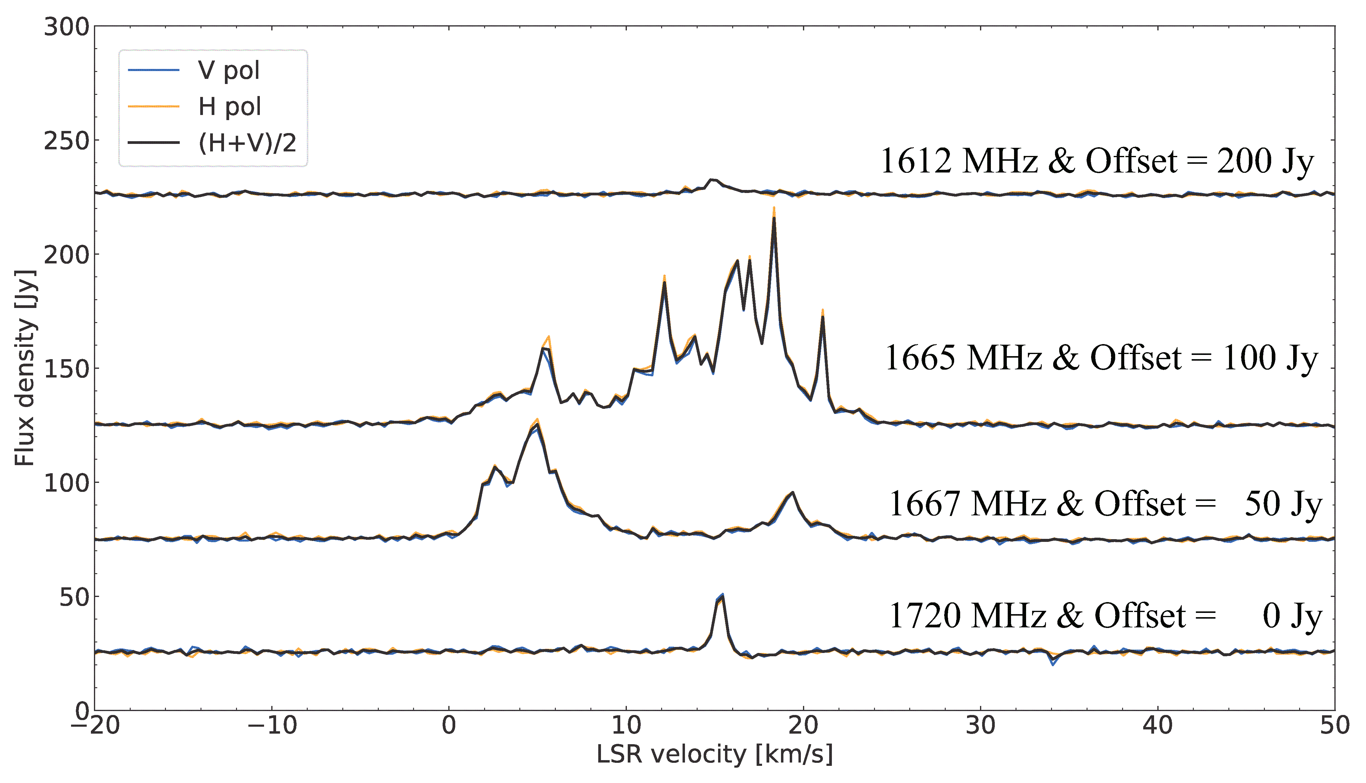
Figure 2-1: OH maser spectra of W49N obtained with 40-m TNRT on 27th November, 2024. Spectra at different transitions of 1612.231 (top), 1665.4018 (top middle), 1667.359 MHz (bottom middle), and 1720.530 (bottom) MHz are shown. For visualization purpose, these spectra are vertically shifted. Note that these spectra include continuum emission (~30 Jy).

Figure 2-2: (Top) OH maser spectra of VY CMa obtained with 40-m TNRT on 30th May, 2024. Spectra at different transitions of 1612.231 (top), 1665.4018 (middle) and 1667.359 MHz (bottom) are displayed. These figures are vertically shifted for visualization. (Bottom) The maximum flux density of each transition is shown as a function of time.
- Alcolea et al. 1999, A&AS, 139, 461
- The Effelsberg-Bonn Hi Survey: Milky Way gas, B. Winkel, J. Kerp, L. Flöer, P. M. W. Kalberla, N. Ben Bekhti, R. Keller and D. Lenz, (2016) A&A 585, A41
- GASS: The Parkes Galactic All-Sky Survey. Update: Improved correction for instrumental effects and new data release, Kalberla, P.M.W. and Haud, U. (2015), A&A, 578, A78
- The Leiden/Argentine/Bonn (LAB) Survey of Galactic HI. Final data release of the combined LDS and IAR surveys with improved stray-radiation corrections, Kalberla, P.M.W., Burton, W.B., Hartmann, Dap, Arnal, E.M., Bajaja, E., Morras, R., & Pöppel, W.G.L. (2005), A&A, 440, 775
- Muders, D., Hafok, H., Wyrowski, F., et al. 2006, A&A, 454, L25
- Useful equations for radio astronomy, credit: Tobias Westmeier
- Williams, D. R. W. 1973, A&AS, 8, 505
- Yudaeva 1986, SvAL, 12, 150