Contents
1. Beam Pattern
2. L-band Pointing Accuracy for 40-m TNRT
3. Amplitude Calibration with Noise Source Injection
4. Aperture Efficiency with its Dependence along Elevation
5. RFI Bird's-eye View Distribution at TNRO Site
6. Skyline Bird's-eye View Maps
7. System noise temperature (Tsys*) for 1.0 – 1.8 GHz
8. Linearity Net in the L-band System
9. Limitation of Integration Time at Each Observation Scanning
11. Sensitivity
12. Overhead
13. Observation Scanning Modes
14. References
The beam pattern of the 40-m TNRT in L-band was measured on 11-12 March, 2024 by observing a strong continuum source M87 (3C274, Virgo A) that is listed by Perley, R. A. & Butler, B. J. (2017, ApJS, 230, 7) into the catalog of compact and flux well-known calibrators. Although M87 is the well-known source showing a diffuse structure with extended radio lobes across an angular size of around 14 arcmin, the compact brightest core in the center that contains the one-sided jet shows an angular size smaller than 5 arcmin. So, M87 could be assumed as a moderate point-like source for a single-dish radio telescope beam in L-band.
Raster scan observations were performed to measure the TNRT L-band beam pattern. A grid spacing of 250 (arcsec), the frequency range between 1.63 and 1.67 GHz, each grid integration time of 10 seconds, were applied for vertical (V) and horizontal (H) linear polarization data. In the observations, OFF source data were obtained in each date at each different EL of 10, 15, 20, 25, 30, 40, 50, and 60 deg. Total-power in 1.63-1.67 GHz was converted into an antenna temperature Ta* [K] via injecting the Noise-Source at each grid scan (see section "Amplitude Calibration with Noise Source Injection" for the Noise-Source temperature and the conversion procedure in detail).
As a result, beam patterns of V and H polarization are represented in a mapping area of 9,000 × 9,000 arcsec2 as shown in Figure 1-1 (Left: 2-dimension, Right: 3-dimension).
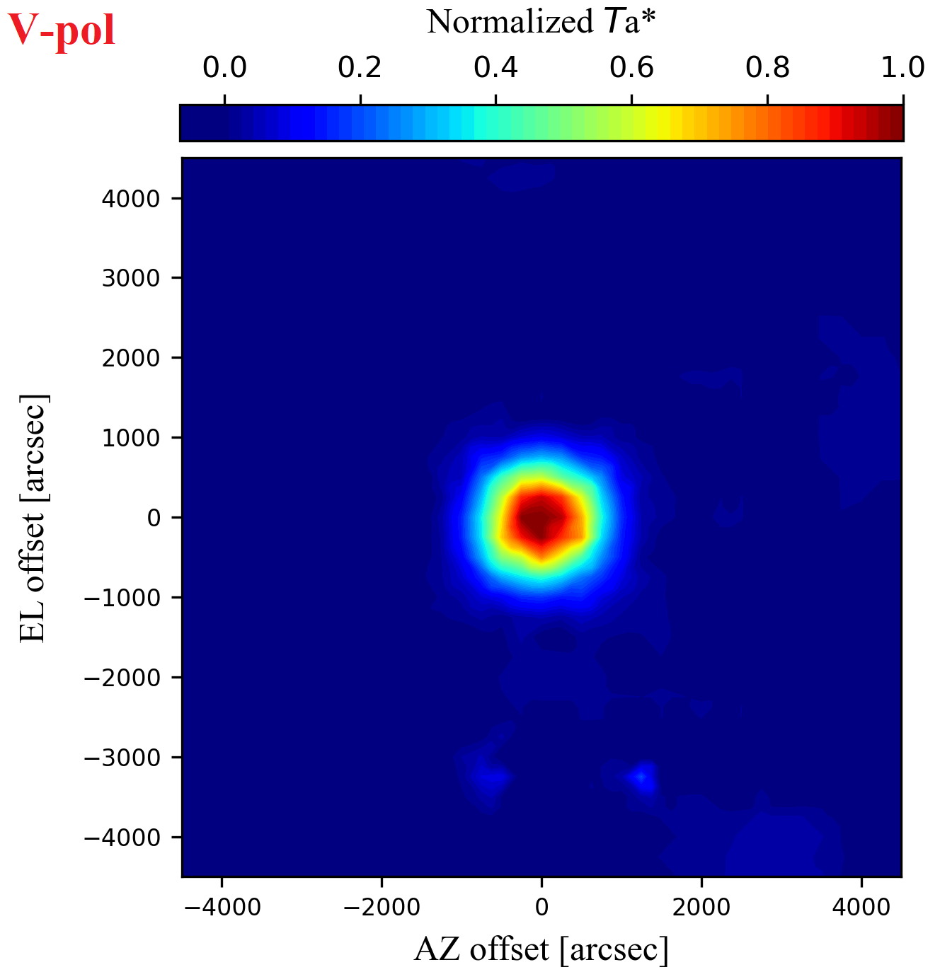
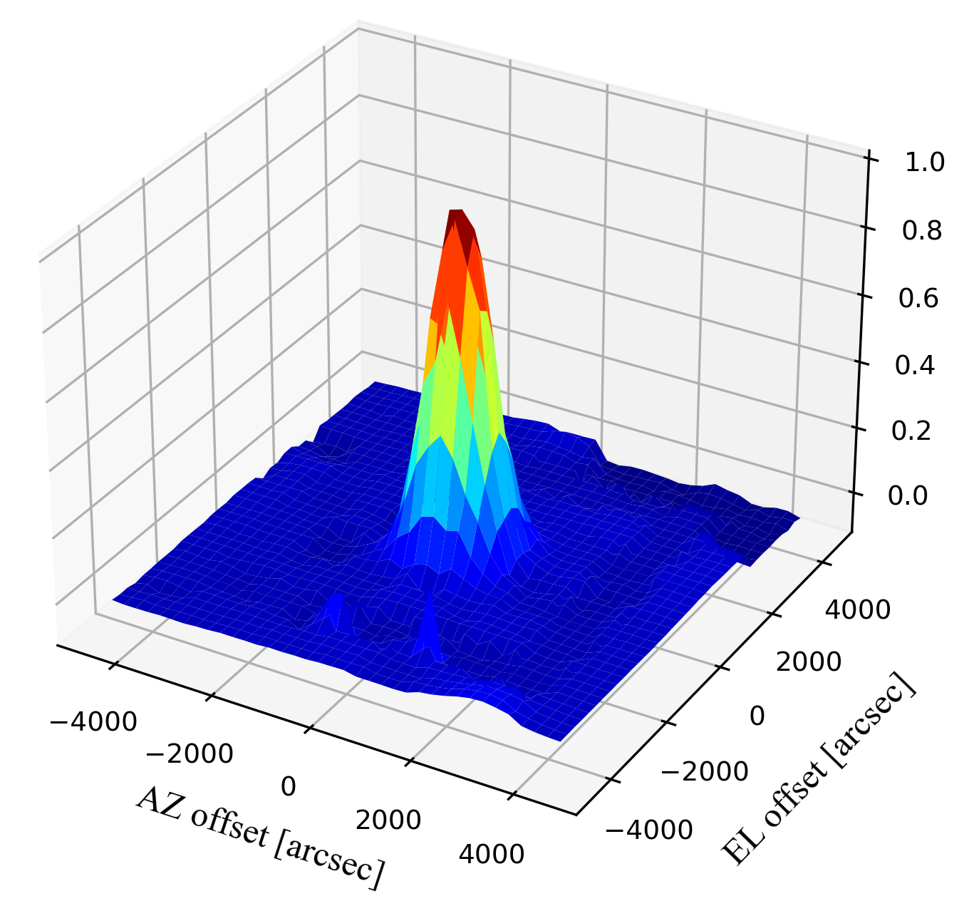
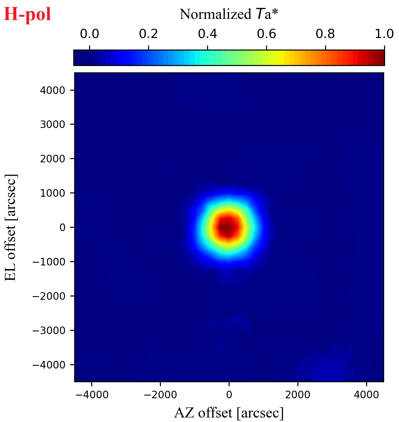
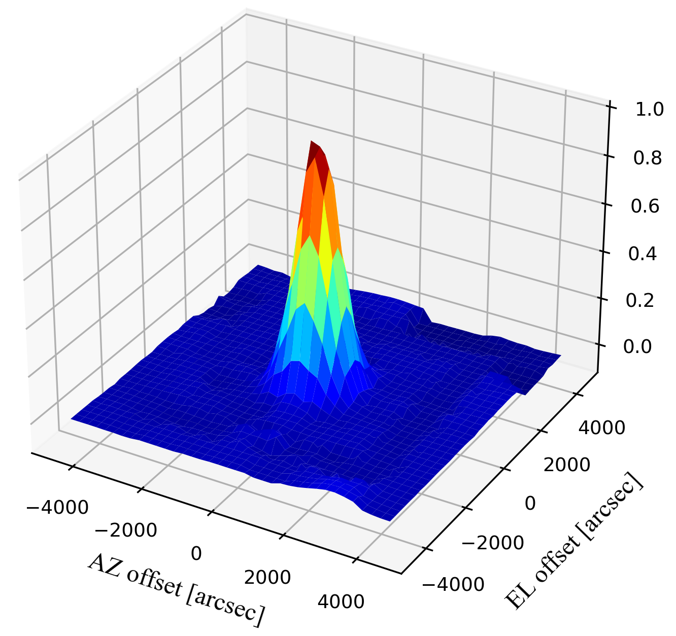
The beam size was quantitatively estimated by fitting the obtained data with a 2-dimensional Gaussian function expressed as follows.
P (∆AZ, ∆EL) = a * exp−4 ln(2)𝜇az − ∆AZHPBWaz2−4 ln(2)𝜇el − ∆ELHPBWel2
where a is the measured brightest antenna temperature, 𝜇az and 𝜇el are pointing offsets in the AZ and EL directions, respectively, and HPBWaz and HPBWel are the half-power beam width in the AZ and EL directions, respectively. The fitting results are shown in Table 1-1. HPBW values are in close agreement with a theoretical value of ~1125 arcsec (i.e., ~1.2 * λ / D where λ and D are the observing wavelength and the diameter of a primary mirror, respectively).
| Type |
Mean ± Standard deviation (arcsec) |
|
|---|---|---|
| V-polarization | H-polarization | |
| HPBWaz | 1,225 ± 7 | 1,217 ± 6 |
| HPBWel | 1,181 ± 6 | 1,214 ± 6 |
| 𝜇az | 3 ± 3 | −29 ± 2 |
| 𝜇el | −45 ± 3 | −25 ± 2 |
2. L-band Pointing Accuracy for 40-m TNRT
• Results
L-band pointing accuracies of TNRT are 30 and 33 (arcsec) in Az and El directions, respectively (see Table 2-1 and Fig. 2-1). The pointing accuracies in Az and El directions correspond to 2.3 % and 2.5 % of the TNRT beam size, respectively. To determine Az and El offsets, we fitted cross scan data with a Gaussian function. As a result, mean values of Half Power Beam Width (HPBW) in Az and El are consistent with TNRT beam sizes in Az and El, respectively, between 1.6-𝜎 and 2.6-𝜎 (see Tables 1-1 and 2-1). It means that pointing calibrators observed are compact. Note that we analyzed horizontal and vertical polarization data separately since the pointing offset depends on polarization.
| Type |
Mean ± Standard deviation (arcsec) |
Nscans |
|---|---|---|
| Az offset | −2 ± 30 | 904 |
| El offset | −4 ± 33 | 904 |
| Az FWHM | 1287 ± 39 | 904 |
| El FWHM | 1297 ± 45 | 904 |
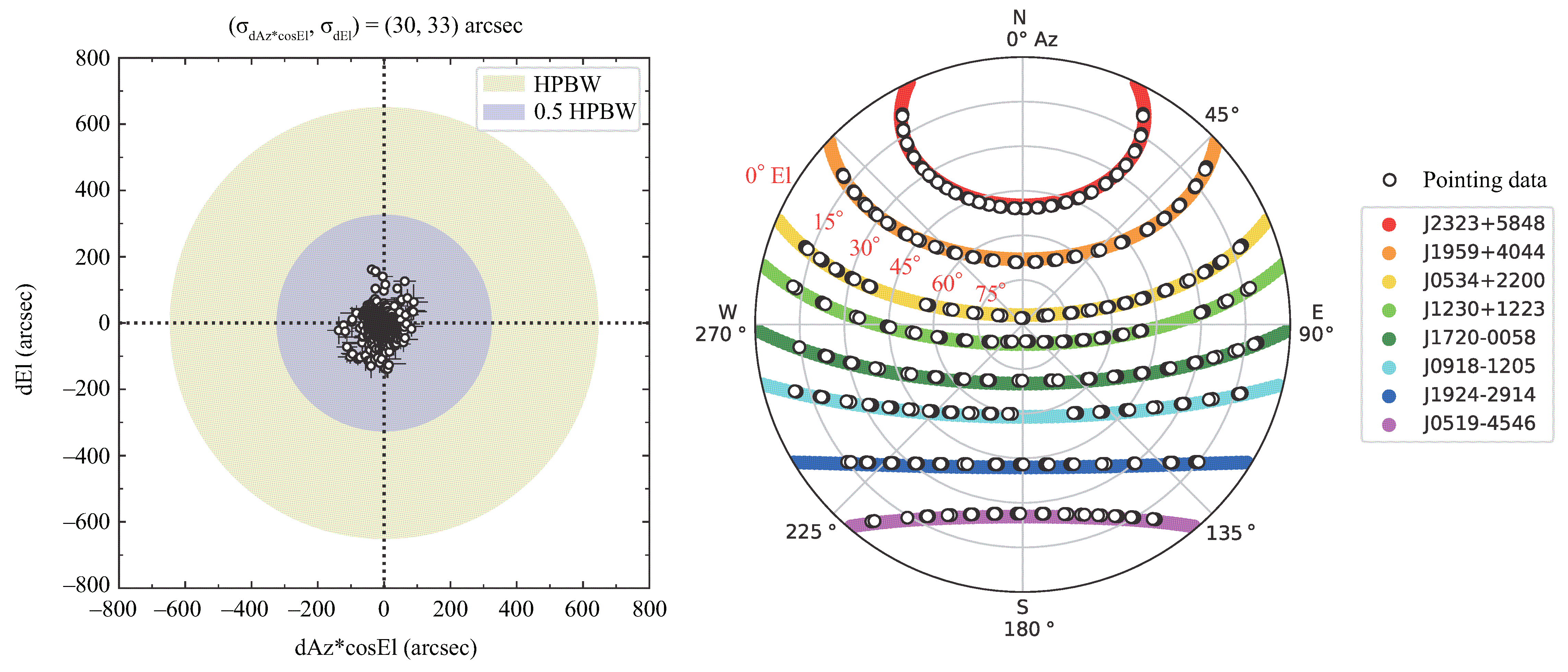
Figure 2-1: (Left) L-band TNRT pointing results, Az offset (dAz*cosEl) and El offset (dEl) values, are shown. The number of data points is 904. Standard deviations of (dAz*cosEl, dEl) are 30 and 33 (arcsec), respectively. Yellow and blue ellipses indicate the Half Power Beam Width (HPBW) and 50% HPBW of TNRT, respectively. (Right) 904 data points (white circles) used in (Left) are plotted on the polar projection of the sky in horizontal coordinates. Note that East is shown in right side, rather than left. We observed eight continuum sources listed by Perley & Butler (2017) and the VLBA Calibrator Search Tool. Individual trajectories of the eight sources are shown by different colors.
• Pointing model
Regarding TNRT pointing model, we referred to de Vicente & Barcia (2007) which introduced a pointing model for Nasmyth telescope. Using the model, Az and El offsets are described as
de Vicente & Barcia (2007) explained physical meanings of individual pointing coefficients/parameters (see Table 2-2).
| Parameter | Physical meaning |
|---|---|
| P1 | Azimuth encoder offset. If positive the antenna always point towards larger azimuth values. This term also includes positioning errors for receivers in the Nasmyth focus. |
| P2 | Collimation error. It includes positioning errors for Nasmyth mirrors. |
| P3 | Lack of orthogonality between the azimuth and elevation axes. If positive both axis form an angle smaller than 90º. This term also includes positioning errors for receivers in the Nasmyth focus. |
| P4 | Tilt of azimuth axis along a E-W direction. If positive the axis is tilted towards the East. |
| P5 | Tilt of azimuth axis along a N-S direction. If positive the axis is tilted towards the South. |
| P4 | Tilt of azimuth axis along a E-W direction and N-S direction. Since it is a combination, the sign does not inform about the direction of the axis tilt. |
| P5 | Tilt of azimuth axis along a N-S direction and E-W direction. Since it is a combination, the sign does not inform about the direction of the axis tilt. |
| P7 | Elevation encoder offset. If positive the antenna always points towards higher elevations. It also includes positioning errors for Nasmyth mirrors. |
| P8 | Gravitational effects. It also includes positioning errors for receivers in the Nasmyth focus. |
| P9 | Gravitational effects. It also includes positioning errors for receivers in the Nasmyth focus. |
• Atmospheric refraction model
The following atmospheric refraction model is applied for observations with 40-m TNRT,
where r0 , b1 and b2 are fixed to be 76.6, 5.7 and 2.3, respectively, based on the annual average of TNRT weather data (i.e., temperature; pressure; relative humidity). We have simulated that pointing errors due to weather changes are up to +/-100 (arcsec) and +/-200 (arcsec) at El = 10 and 5 deg, respectively. These errors correspond to 7.8% and 15.6% of the TNRT beam size at L-band, respectively. Pointing errors due to the weather changes are < 50 (arcsec) at high El > 20 deg.
• Pointing procedures
Firstly, we determined only large constant offsets (i.e., P1 and P7) by observing one or two bright calibrators (e.g., J2323+5848 = Cas-A; J1959+4044 = Cyg-A; ) listed by Perley & Butler (2017). During pointing observations, we conducted cross scans in Az and El directions with each scan length of 10,560 (arcsec). 112 data points with each integration time of 0.536 (sec) were applied for each Az or El scan, which gives a spatial spacing between individual data points of 94 (arcsec). Also, we recorded radio frequency between 1630 and 1670 MHz with a frequency resolution of 200 (kHz) during the pointing observations. The frequency range is relatively Radio Frequency Interference (RFI) quiet in the TNRT L-band observation.
Secondly, we observed eight pointing calibrators covering a wide range of Az and El (see Fig. 2-1) so that we can determine all pointing parameters (P1, P2, P3, P4, P5, P7, P8, P9). Narrower cross scans, having each scan length of 5000 (arcsec) and a spatial spacing of 89 (arcsec), were applied. The data integration time was increased from 0.536 (sec) to 1.074 (sec).
Lastly, we observed the same calibrators with the pointing parameters determined above so that we can evaluate the pointing accuracy of TNRT (see Table 2-1).
3. Amplitude Calibration with Noise Source Injection
Conversion of total power into an antenna temperature for the amplitude calibration in the TNRT L-band system is achieved by injecting a noise source (NS). The injection of this NS consists of each sub-scan with this percentage: NS-ON 0.25% and NS-OFF 99.75%. So, for example, each accumulation period of each subscan data of 1 sec gives us NS-ON 0.0025 sec (to be used for calibration) & NS-OFF 0.9975 sec (to be used for integration to detect an astronomical object). However, both of them show the same time stamp.
The system noise temperature Tsys* can be calculated by (1) injecting a NS or (2) the Chopper wheel method (e.g., see Ulich & Haas 1976) as follows:
Tsys* =TNSPsky+NSPsky − 1 exp(𝜏(El)) (3-1)
Tsys* =TambPRPsky − 1 (3-2) Chopper wheel method
where TNS and Tamb are temperatures of NS [K] and the ambience, respectively, Psky+NS and Psky are the observed powers with and without injecting NS, respectively, PR is the radio power of an absorber whose temperature is consistent with Tamb, and 𝜏 is an optical depth. The essential factor TNS in the TNRT L-band was practically determined by temporarily attaching an absorber to the horn, allowing us to observe black body emission at a temperature equivalent to the ambient temperature. This was done using the secZ method according to the following equations:
ln (Tsys* + Tamb) = 𝜏0 secZ + ln (Trx + Tamb + Tbg) (3-3)
TNS = (Trx + Tamb) PR+NSPR − 1 (3-4)
where Trx and Tbg (= 2.7 K) are temperatures of the receiver and the background, respectively, and PR+ns and PR are the observed powers when the horn is covered with the absorber with and without NS injection, respectively. 𝜏0 is an optical depth at zenith. By plotting ln (Tsys* + Tamb) against secZ (= 1 / sin El), we can determine 𝜏0 and ln (Trx + Tamb + Tbg) from the slope and intercept of the plot. Note that Tsys* can be determined using the Chopper wheel method. Lastly, we can determine the noise source temperature TNS of the TNRT L-band receiver from Eq. (3-4).
As a result, TNS was determined to be 31.9 ± 0.4 K, while 𝜏0 was estimated to be 0.0106 ± 0.0019 as a bi-product. The new TNS value falls well within the uncertainty of the previous determination (30.9 ± 1.1 K) and is a considerable improvement to the estimate.
Verification of this TNS was completed by comparing Tsys* measurements obtained by injecting the NS with those obtained using the R-Sky method with the absorber. Here, we determined Tsys* using the new TNS and the measured powers in the frequency ranges 1630 - 1670 MHz (no line emission) and 1425 - 1445 MHz (close to the HI line). Along the secZ axis, Tsys* consistently ranged between 18 and 32 K within 10% errors using either of the methods in the 1630 - 1670 MHz range on three different tracks at AZ = 300, 315 and 330 deg, as shown in Figure 3-1 (NS: red, R-Sky: blue).
Similar results were also achieved when considering 1425 - 1445 MHz (Figure 3-2). Although the NS method yields systematically lower Tsys* (2 - 3 K) compared to the R-sky method, they are generally within 1σ of one another and are therefore acceptable. Note also that Tsys* determined at (AZ, EL) = (315, 80) deg is an outlier due to possible RFI signals (see Section 6 for skyline bird's-eye view maps). The best Tsys* of around 17.5 K demonstrates that this L-band receiver developed in collaboration with MPIfR (Gundolf Wieching et al.) is one of the best low-noise sensitive receivers in the world.
At the end, an antenna temperature Ta* can be calculated as follows:
Ta* = Tsys* PonPoff − 1
where Pon and Poff are observed power of ON astronomical source and OFF source (Sky), respectively.
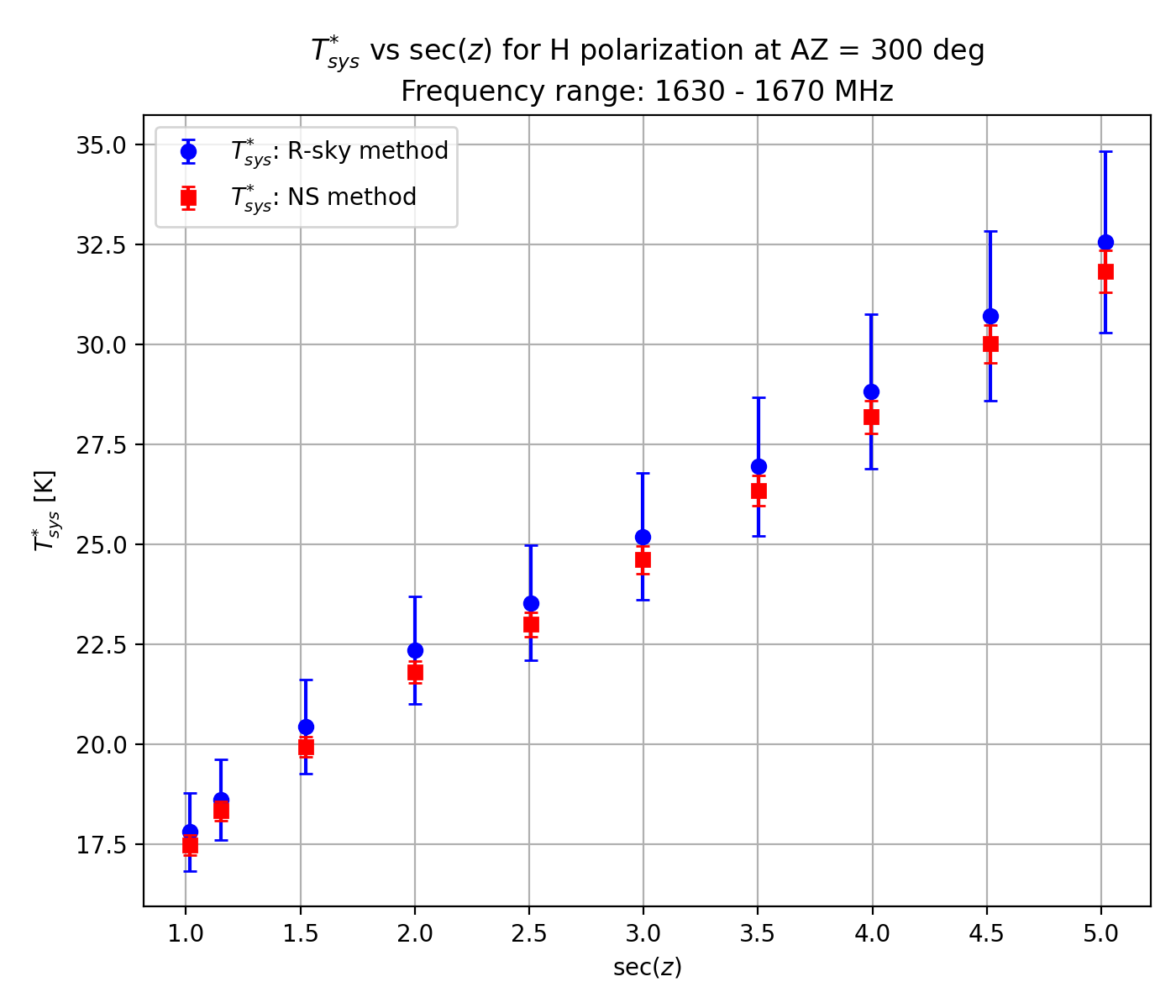


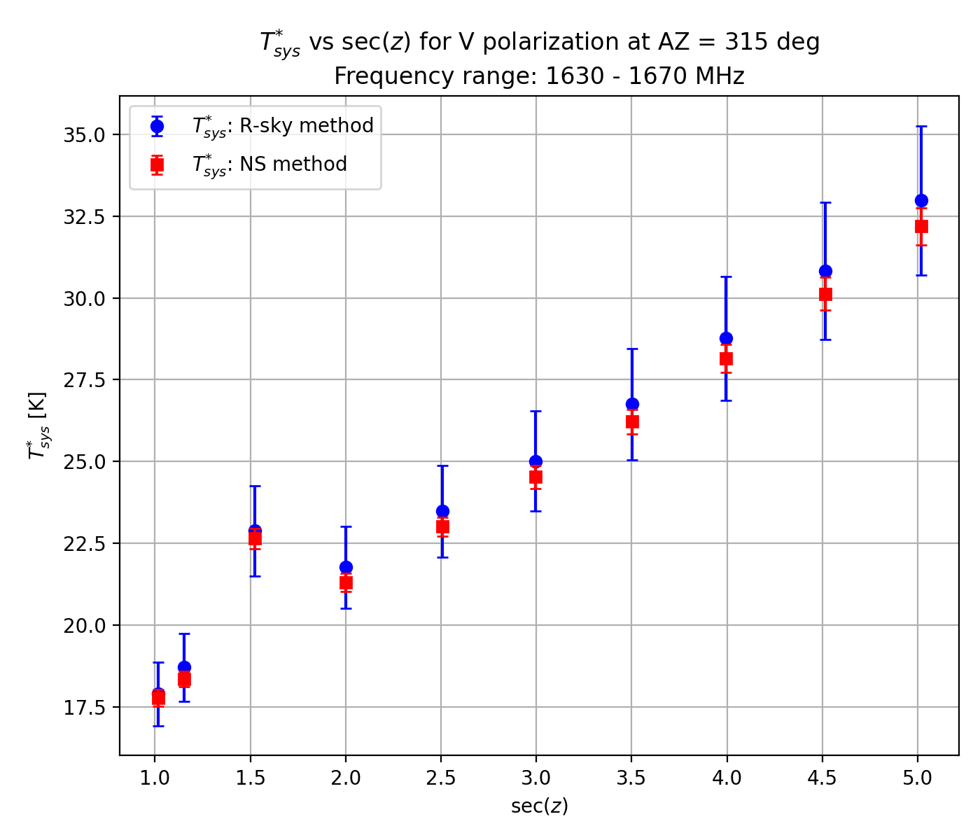
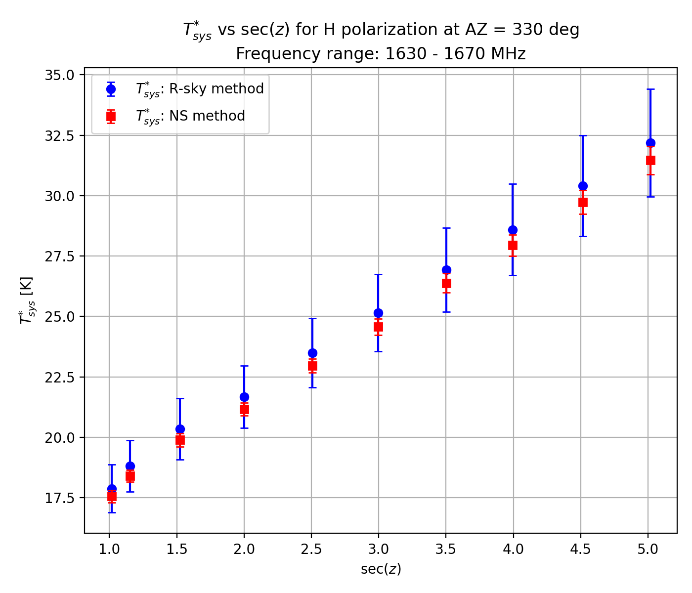

Figure 3-1: System noise temperature Tsys* versus secZ using the noise source and R-sky methods (shown by red and blue circle symbols, respectively). The frequency range of interest here is 1630 - 1670 MHz. Three different tracks of AZ = 300 (top), 315 (middle) and 330 deg (right) are considered.
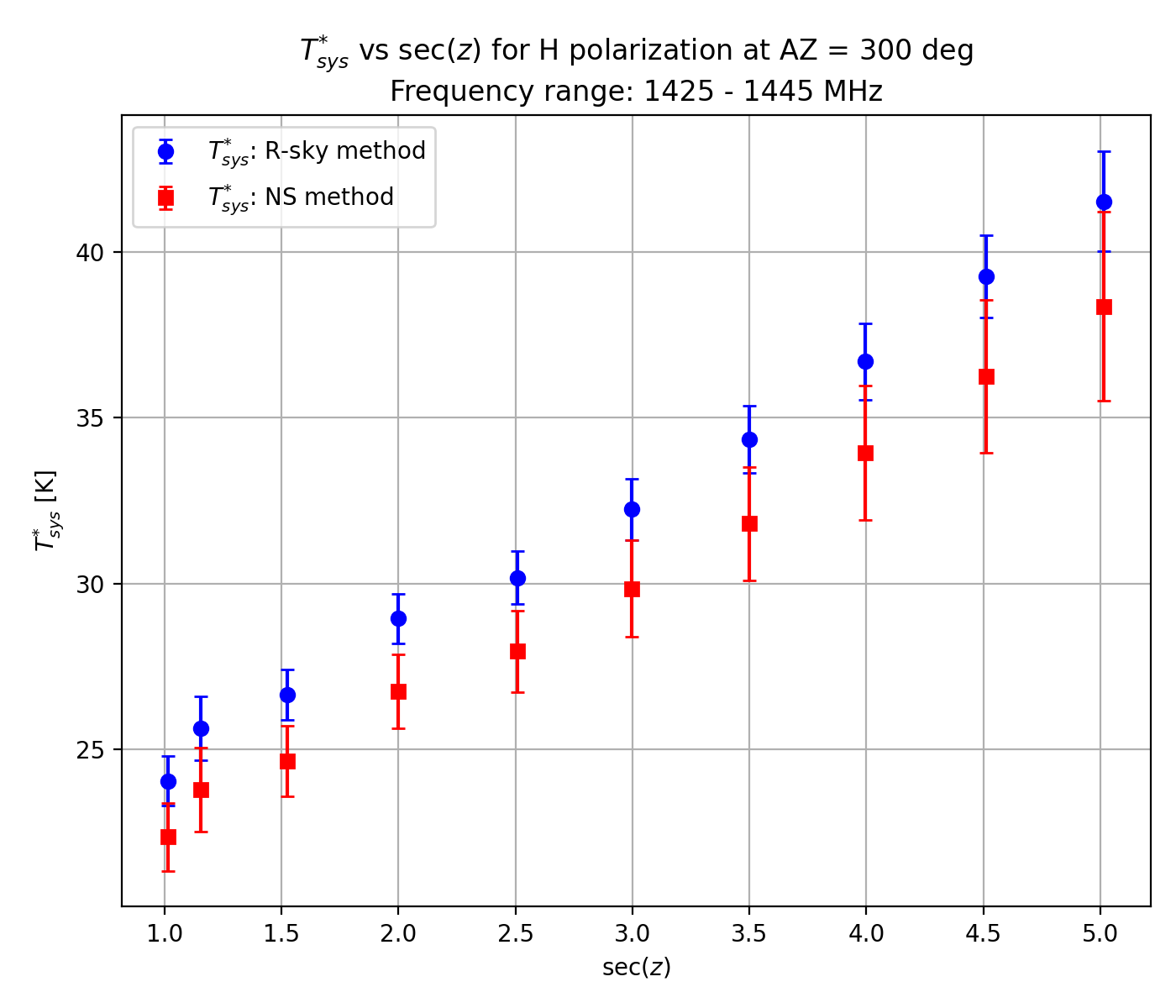


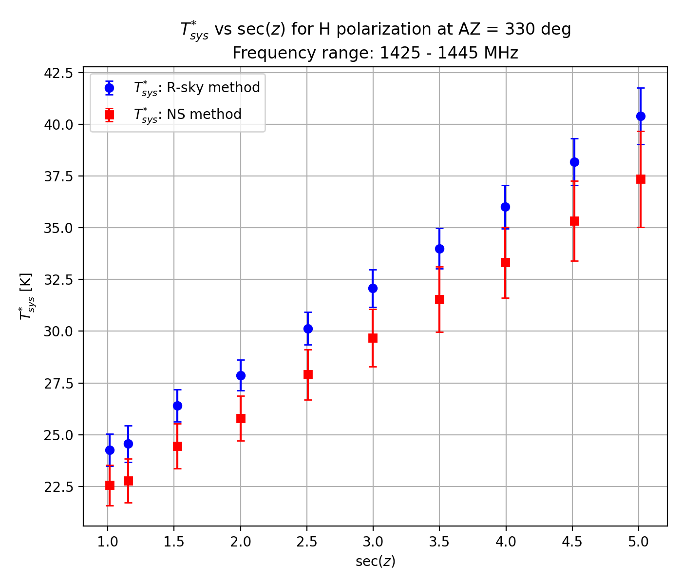

Figure 3-2: System noise temperature Tsys* versus secZ using the noise source and the R-sky methods (shown by red and blue circle symbols, respectively). The frequency range of interest here is 1425 - 1445 MHz. The same tracks of AZ = 300 (top), 315 (middle) and 330 deg (right) are considered.
4. Aperture Efficiency with its Dependence along Elevation
The aperture efficiency of the TNRT L-band system, in which the receiver is installed at the prime focus, was measured in February–March 2024 for dual linear polarizations by observing strong and moderate / complete compact continuum calibrators whose flux densities with its stability in L-band are well-known as listed in Perley, R. A. & Butler, B. J. (2017, ApJS, 230, 7): we selected two sources M87 (3C274, Virgo A) and J0437+2940 (3C123). These calibrators cover the wide range of the elevation angles, resulting in determining dependence of the aperture efficiency along elevation. Toward the data integrated in frequency range of 1.63-1.67 GHz that is the range without any noticeable disruptive RFI signals and is close to the rest frequencies of ground-state OH masers, the best fit results of the elevation dependence with a cubic function for vertical and horizontal linear polarizations 𝜂A_V(EL) and 𝜂A_H(EL), respectively, are as follows:
𝜂A_V(EL) = 8.13 × 10⁻⁸ EL3 −1.84 × 10⁻⁵ EL2 + 1.43 × 10⁻³ EL + 0.504
𝜂A_H(EL) = 3.32 × 10⁻⁷ EL3 −5.53 × 10⁻⁵ EL2 + 2.89 × 10⁻³ EL + 0.471
and as shown in figure 4-1. The aperture efficiencies are stable as 51.6-54.3% and 49.5-52.5% for the vertical and horizontal linear polarizations, respectively, in elevation higher than +10 deg.
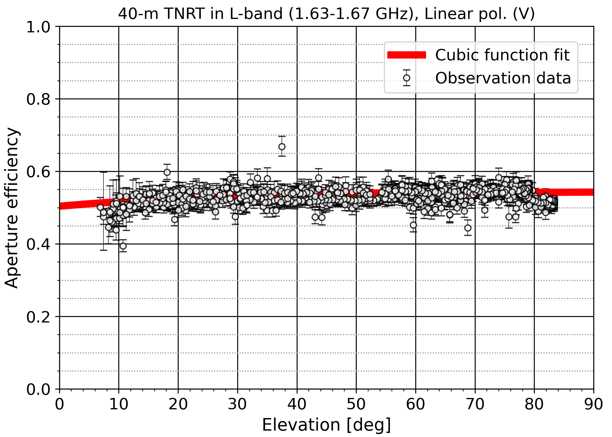

Figure 4-1: Aperture efficiency of the TNRT L-band measured in 1.63-1.67 GHz for vertical (left-panel) and horizontal (right-panel) linear polarizations with its dependence along elevation. The red and blue curve line presents the best fit on the observation data by a cubic function for vertical and horizontal linear polarization: 𝜂A_V(EL) = 8.13 × 10⁻⁸ EL3 −1.84 × 10⁻⁵ EL2 + 1.43 × 10⁻³ EL + 0.504, and 𝜂A_H(EL) = 3.32 × 10⁻⁷ EL3 −5.53 × 10⁻⁵ EL2 + 2.89 × 10⁻³ EL + 0.471, respectively.
Evaluations of the elevation dependence with a cubic function were also conducted in frequency range of 1.425-1.445 GHz that is near the rest frequency of 21-cm HI line emission, as shown in figure 4-2. The range of aperture efficiencies is 53.4-59.3% and 52.5-57.3% for the vertical and horizontal linear polarizations, respectively, in elevation higher than +10 deg. These ranges are approximately two times wider than the case integrated in 1.63-1.67 GHz, which might be caused by lower signal-to-noise ratios on the data integrated in 1.425-1.445 GHz due to the presence of more RFI signals.
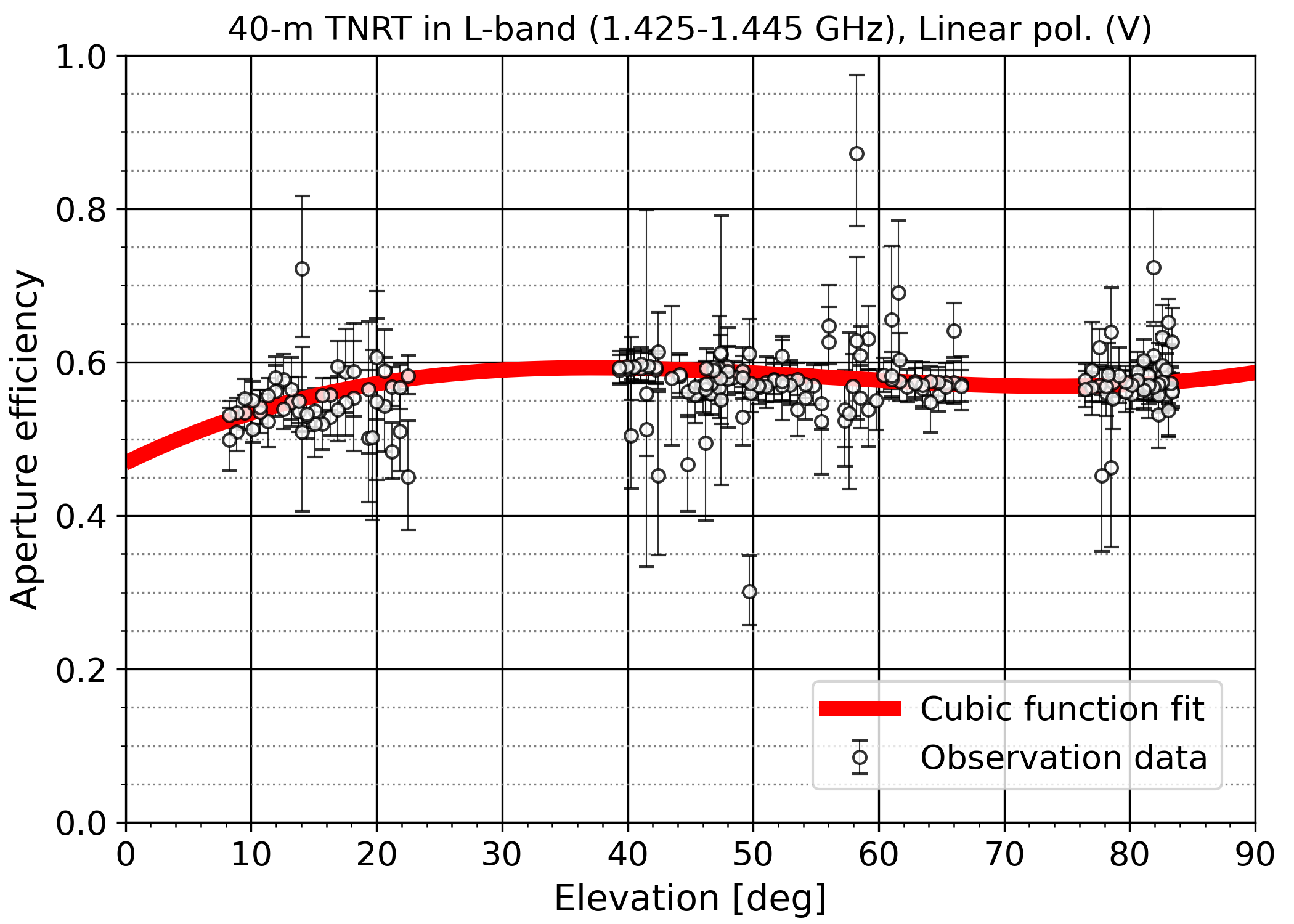

Figure 4-2: Aperture efficiency of the TNRT L-band measured in 1.425-1.445 GHz for vertical (left-panel) and horizontal (right-panel) linear polarizations with its dependence along elevation. The red and blue curve line presents the best fit on the observation data by a cubic function for vertical and horizontal linear polarization: 𝜂A_V(EL) = 9.73 × 10⁻⁷ EL3 −1.62 × 10⁻⁴ EL2 + 8.02 × 10⁻³ EL + 0.469, and 𝜂A_H(EL) = 7.37 × 10⁻⁷ EL3 −1.20 × 10⁻⁴ EL2 + 5.88 × 10⁻³ EL + 0.477, respectively.
5. RFI Bird's-eye View Distribution at TNRO Site
To mitigate especially strong RFI impacts on the TNRT L-band system at the telescope site, a 90 cm parabolic reflector antenna (Rohde & Schwarz AC008 with HL024A1) was temporary installed at the top of the GNSS tower, which is located 40 m away from the TNRT in the North-East direction, as shown in figure 5-1. It enabled us to watch the same sky of TNRT for the RFI investigation with the 90-cm telescope. The 1st trial of this RFI investigation was completed in March 2023. The observation data were recorded by using Keysight Fieldfox N9918B Spectrum analyzer in the frequency range of 1-2 GHz with a frequency resolution of 100 kHz. Both the max hold and averaged values over 30 sec integration were recorded. These data were obtained at each 3 deg steps both in AZ and EL directions, resulting in the 1st release of a RFI bird's-eye view map for L-band at the telescope site, as shown in figure 5-2 (right).
This map constructed with total-power averaged over 30 sec and summed in 1-2 GHz frequency range presents that the power rises up to around 5 dB everywhere except for areas of EL higher than 45 deg and a part of the North-West direction. However, in the South-East direction at EL lower than 15 deg, we would like to emphasize that the super-strong RFI monster obstructs any observations due to super saturation of the L-band system, which might break the L-band receiver itself, in particular for the AZ range of 130-170 deg with rising the total-power up around 15 dB. Based on detailed investigations with spectra, e.g., figure 5-2 (left), a major contributor of those RFI monsters corresponds to a strong radio signal in 1.805-1.845 GHz, which could be caused by mobile base stations surrounding the telescope site.
In this CfP cycle, we have a plan to overcome this issue by avoiding those dangerous RFI monster zones via implementing a dynamic scheduling with other target sources and/or flagging at post-processing.
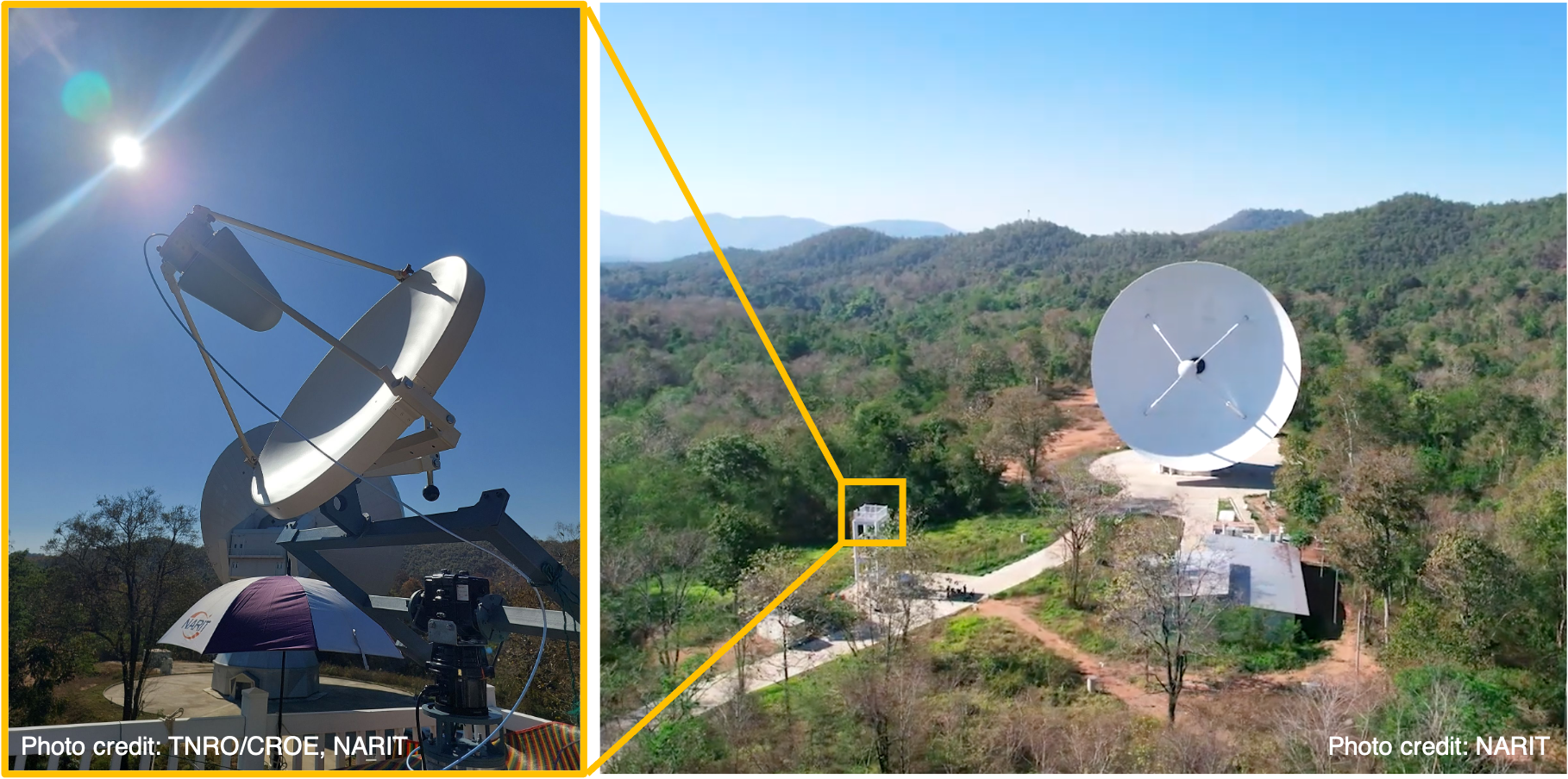
Figure 5-1: The 90 cm parabolic reflector antenna (left) installed at the top of the GNSS tower, which is located 40 m away from the TNRT in the North-East direction (right).
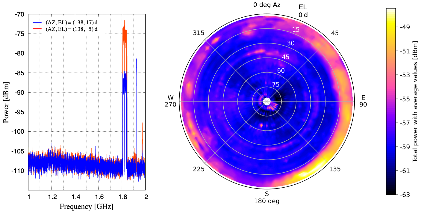
Figure 5-2: (Right) RFI bird's-eye view map observed with the 90 cm parabolic reflector antenna. Color code represents a total-power averaged over 30 sec and summed in 1-2 GHz frequency range in the unit of dBm (see the color scale in the right-hand side bar). (Left) An example of averaged spectra observed at (AZ, EL) = (138, 17) and (138, 5) deg shown by blue and red solid lines, respectively.
6. Skyline Bird's-eye View Maps
For practical observations with the 40-m TNRT in the usable frequency range of this CfP cycle, 1.0 – 1.8 GHz with the dual linear polarization, skyline bird's-eye view maps obtained by 40-m TNRT observations are released as shown in figures 6-1, 6-2, and 6-3. These maps clarify obstacles for TNRT observations. For making the maps, TNRT observations were conducted in March 2024 where the whole sky of AZ = 0 – 360 deg and EL = 4 – 85 deg was mapped with 5 and 2 deg angle steps for Az and El, respectively. Vertical and horizontal linear polarization data were integrated in different frequency ranges (see figures 6-1, 6-2, and 6-3) over 10 sec at each (Az, El) position. The integrated total-power data were converted to system noise temperatures [K] with the Noise-source injecting method.
Figure 6-1 represents skyline bird's-eye view maps for TNRT observations of satellite and main lines of OH masers. The main lines of OH masers (1665 and 1667 MHz) can be observed with low Tsys* values (< ~50 K) at high El > ~15 deg. However, we can see very high Tsys* values (> ~500 K) at (Az, El) = (Az = ~160 – ~180, El < 15) deg. An observer should avoid that region from TNRT observations. Tsys* values are slightly increased for a satellite line of OH maser at a rest frequency of 1612.231 MHz, compared to the main lines of OH masers. TNRT observation for a satellite line of OH maser at a rest frequency of 1720.530 MHz is affected by higher Tsys* values compared to the other lines of OH masers. We can see high Tsys* values (> ~200 K) as radial pattern at high El > 60 deg and arc pattern at El < 45 deg in Figure 6-1 (bottom).
Figure 6-2 displays skyline bird's-eye view maps (dual polarization) for the frequency range of H I (i.e., within 1420.405 +/- 2.5 MHz and VLSR +/- ~500 km s-1). Since H I is bright and detected over entire the sky, some Tsys* values are overestimated due to the H I emission (a few Kelvin or more). Observation areas with good Tsys* values (< ~30 K) are very limited for H I observations. However, we have confirmed that H I observation is possible for scientific purposes (see more detail in the "Science Commissioning" of this web page).
Figure 6-3 shows skyline bird's-eye view maps (dual polarization) for the full frequency range of TNRT L-band receiver, 1,000 – 1,800 MHz.
We recommend applicants to refer to the following Skyline Bird's-eye view maps for the sensitivity calculation and scheduling of science observations.
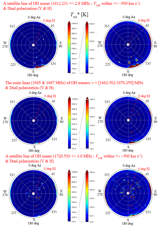
Figure 6-1: (Top row) Skyline bird's-eye view maps (dual linear polarization) obtained by 40-m TNRT L-band observations for a satellite line of OH maser at a rest frequency of 1612.231 MHz. Tsys* values were determined for the frequency range, 1612.231 +/- 2.8 MHz, corresponding to the LSR velocity range within VLSR +/- ~500 km s-1. Different Tsys* ranges, Tsys* = 15 - 1,000 K (left) and 15 - 300 K (right), are used for color bars. Tsys* beyond the maximum value is shown by deep red. (Middle row) Similar to the top row, but for the main lines of OH masers at rest frequencies of 1665.4018 and 1667.359 MHz. The frequency range of the maps is 1662.5018 – 1670.259 MHz. (Bottom row) Similar to the top row, but for a satellite line of OH maser at a rest frequency of 1720.530 MHz. Frequency range is 1720.530 +/- 3.0 MHz, corresponding to the LSR velocity range VLSR +/- ~500 km s-1.

Figure 6-2: Skyline bird's-eye view maps for an H I frequency range (within 1420.405 +/- 2.5 MHz and VLSR +/- ~500 km s-1) of dual linear polarization. Color codes represent Tsys* [K] in the ranges of Tsys* 15 - 1,000 K (left) and 15 - 300 K (right), respectively. Tsys* beyond the maximum value is shown by deep red.

Figure 6-3: Skyline bird's-eye view maps for the full frequency range (1.0 – 1.8 GHz) of dual linear polarization. Color codes represent Tsys* [K] in the ranges of Tsys* 15 - 1,000 K (left) and 15 - 300 K (right), respectively. Tsys* beyond the maximum value is shown by deep red.
7. System noise temperature (Tsys*) for 1.0 – 1.8 GHz
Using the same data as in "6. Skyline Bird's-eye View Maps", we show the opacity corrected system noise temperature Tsys* as a function of frequency. Figure 7-1 shows Tsys* vs. frequency (1–1.8 GHz) for vertical and horizontal polarization in the RFI quiet region at (Az, El) = (341, 60) deg, while Figure 7-2 is the same as Figure 7-1, but for the RFI loud region at (Az, El) = (171, 12) deg. We note that Figure 7-2 corresponds to the prohibited area of TNRT L-band observation explained in "6. Skyline Bird's-eye View Maps".
Figure 7-1 is a reference diagram for observing spectral lines and continuum sources with the 40-m TNRT at L-band.
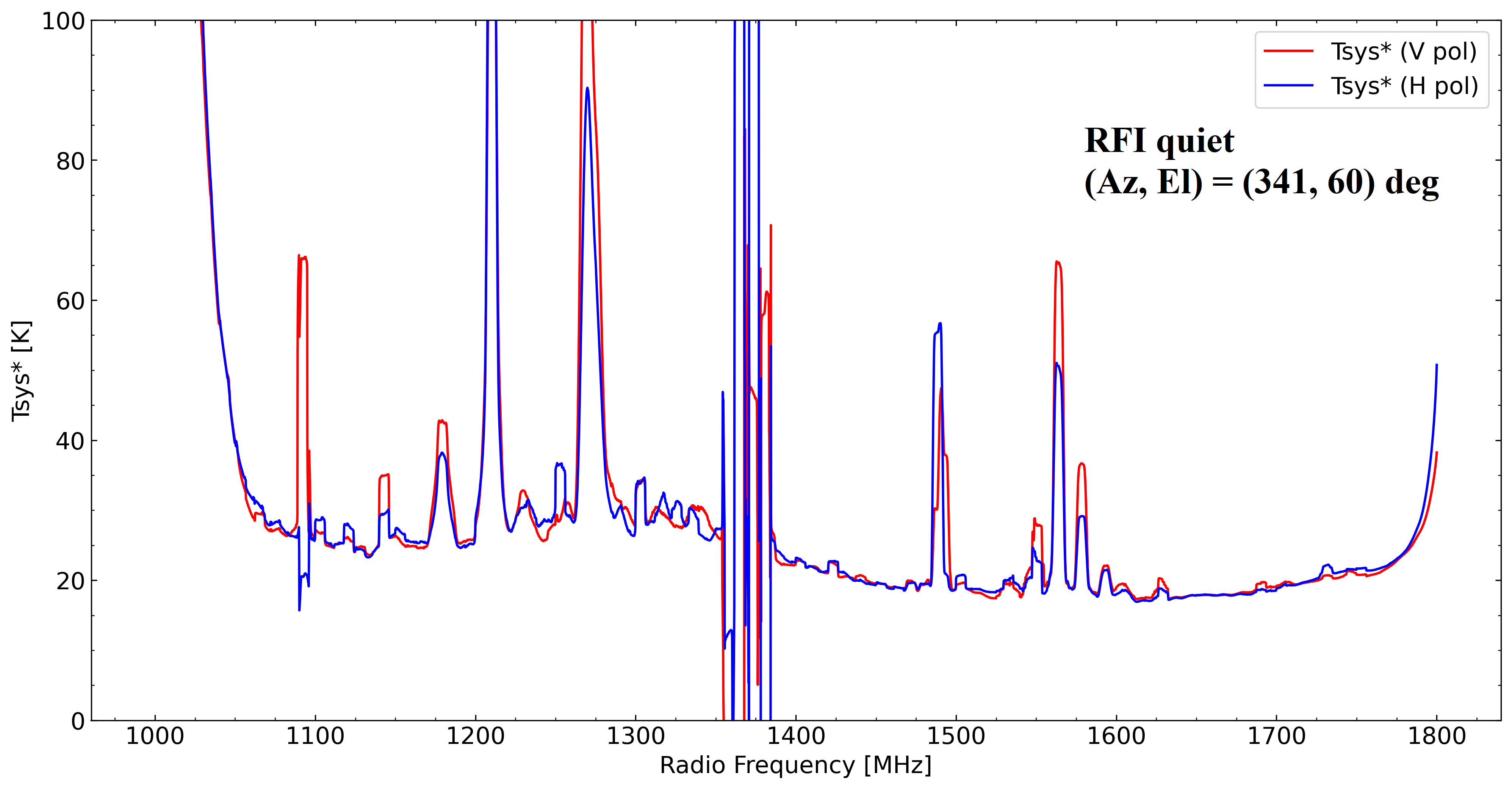
Figure 7-1: The opacity corrected system noise temperature Tsys* is shown as a function of radio frequency (1–1.8 GHz) for the RFI quiet region at (Az, El) = (341, 60) deg. Red and blue represent vertical and horizontal polarization, respectively. The moving average of Tsys* is displayed with a frequency window of 10 MHz.
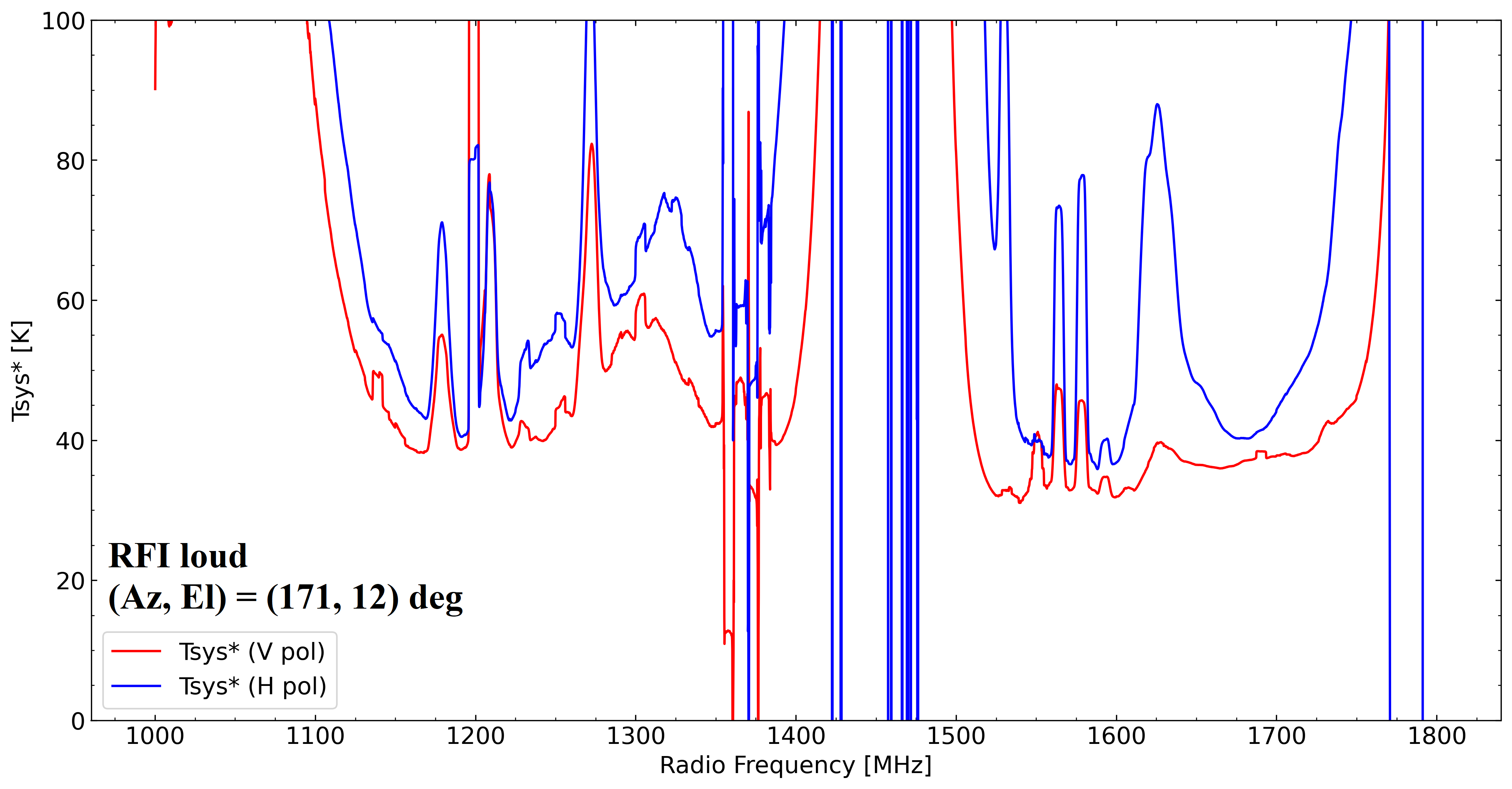
Figure 7-2: Same as Figure 7-1, but for the RFI loud region at (Az, El) = (171, 12) deg.
8. Linearity Net in the L-band System
With the upgraded L-band receiver (now with new bandpass filters to mitigate strong RFI impacts), the linearity with its dynamic range net in the current TNRT L-band system was measured on 26 December 2023. This investigation was completed by observing RFI quiescent / moderate blank sky areas in the following directions: (AZ, EL) = (45, 30), (135, 30), (225, 15), (225, 30), (315, 15), (315, 30) and (315, 60) deg. The observations were achieved by controlling the Digital Step Attenuator (DSA: situated between the 3rd and 4th amplifier in the L-band receiver box) from +30 dB (maximum) to +15 dB, in 1 dB increments. We then averaged the output power over a frequency range for both vertical (V) and horizontal (H) linear polarizations. Here, we defined the uncertainty in power to be 3 times the standard deviation of the power within the chosen frequency range.
Figure 8-1 presents plots of output power against attenuation in dB in the current TNRT L-band system measured in the 1.630 - 1.670 GHz range, where no emission lines were detected, towards the aforementioned (AZ, EL). These results show that the upgraded system can now maintain linearity up to ~10 dB (i.e. 20 - 30 dB) in most cases, marking a significant improvement from Cycle 0 (max. 5 dB between 26 - 30 dB). It is of note that linearity in the V polarization towards (135, 30) and (315, 30) deg is broken at ~23 dB, roughly 3 dB higher than in the H polarization. We attribute this finding to potentially strong V-polarized RFI signals in these directions during observation.
Figure 8-2 shows another set of output power vs attenuation plots (in dB) measured between 1.417 - 1.423 GHz (i.e. HI skyline mapping, see Figure 6-2) at the same directions of (AZ, EL). At these frequencies, the ability to maintain linearity is more dependent on the directions in which observations were taken. Discrepancies between V and H polarizations are also seen in some directions, e.g. (45, 30) and (135, 30) deg, so observers are encouraged to estimate the effects of such results on any polarized emission targets near 1.4 GHz. In areas with minimal to no RFI, a similar dynamic range of 10 dB is achieved in 1.417 - 1.423 GHz. At (45, 30), (135, 30) and (225, 30) deg, less ideal linearity is preserved in the V polarization until attenuation of 22, 24 and 21 dB, respectively, roughly 1-2 dB above the H polarization. Note also that linearity in the V polarization towards (315, 30) deg is questionable, but the H polarization results show excellent linearity down to 18 dB, i.e. 12-dB dynamic range.
Assuming that Tsys* = 20 K and the aperture efficiency = 50%, (Pon − Psky) of 10 dB corresponds to a flux density of around 790 Jy. However, we have checked that observations of bright sources e.g. Cas A and Cyg A (> 1000 Jy) were possible without breaking linearity. Therefore, we confirm that most radio continuum targets are observable with the upgraded L-band at TNRT. Observers are reminded that any observations with the continuum mode must remain within the linear regime to avoid reaching the saturation level, which would yield unreliable reduced absolute flux density. Conversely, there are no restrictions on observing line emissions, such as masers, within this dynamic range of linearity.
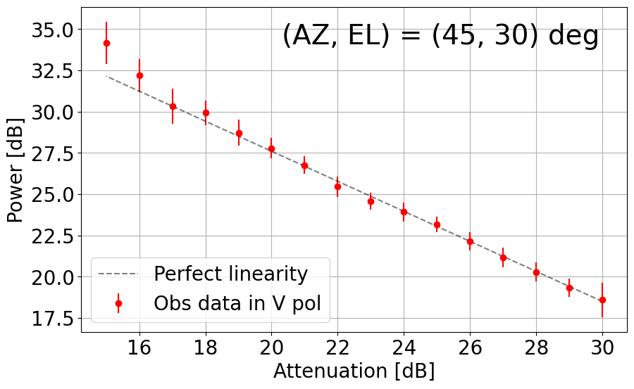


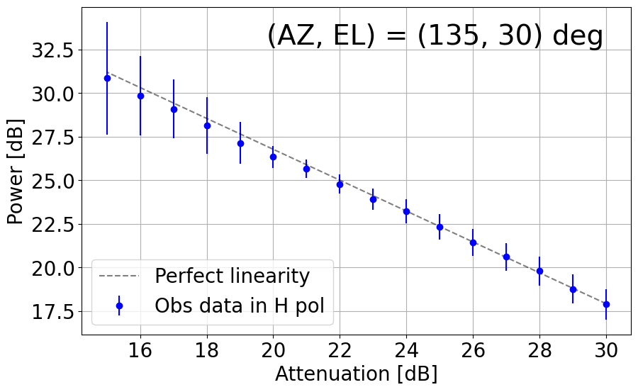


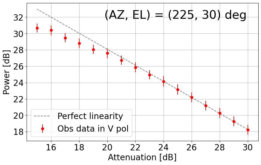
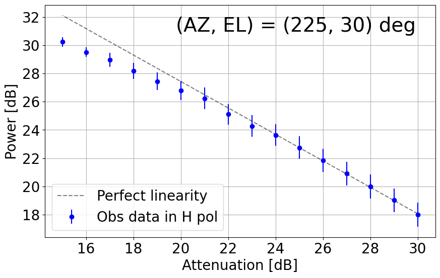
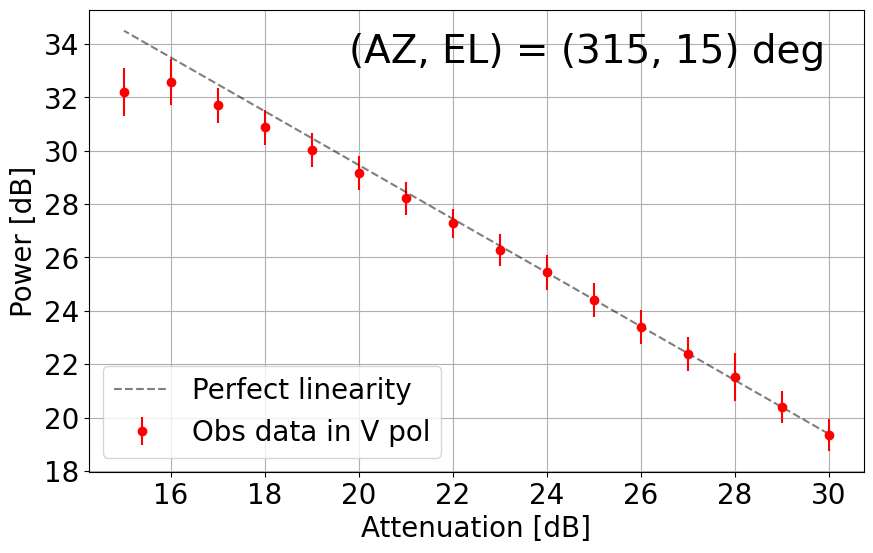
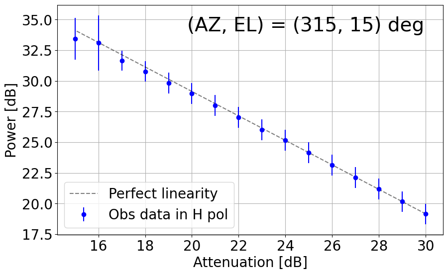
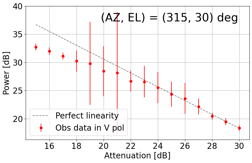


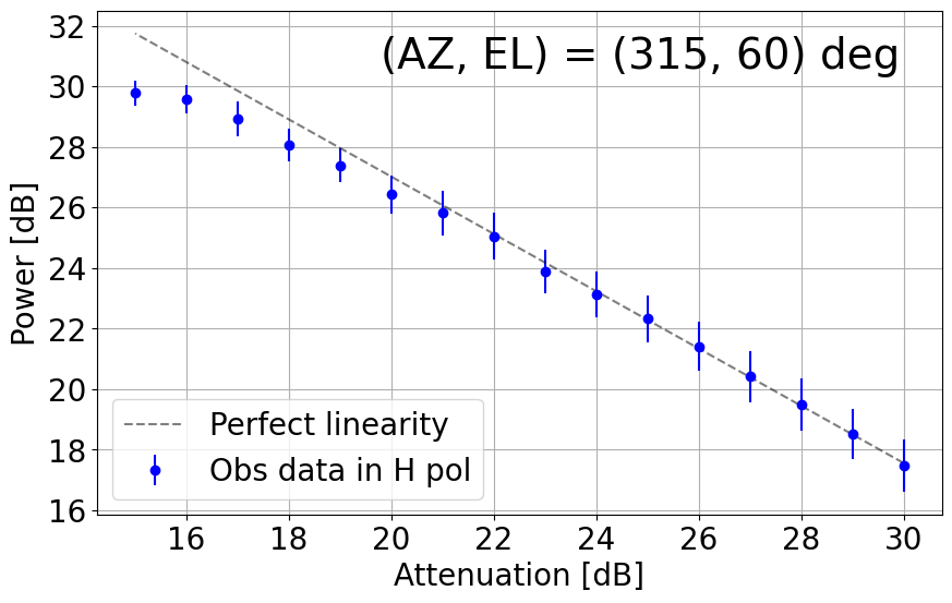
Figure 8-1: Results of linearity investigations in the current TNRT L-band system measured in the 1.630 - 1.670 GHz range for vertical (V, left) and horizontal (H, right) linear polarizations at (AZ, EL) = (45, 30), (135, 30), (225, 15), (225, 30), (315, 15), (315, 30) and (315, 60) deg. Each panel is labelled with the direction in which the measurements were taken. This investigation was completed between attenuation of 15 - 30 dB. The average power at each attenuation is denoted by a filled red (V) or blue (H) circle with its error bar corresponding to 3 times the standard deviation of power. The dashed line in each panel represents perfect linearity within this 16 dB range.

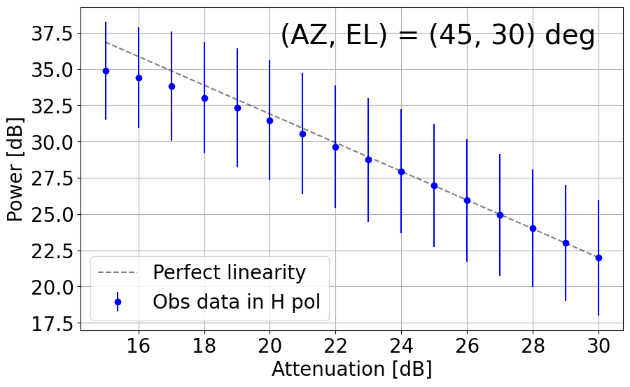

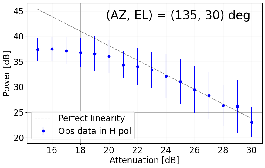
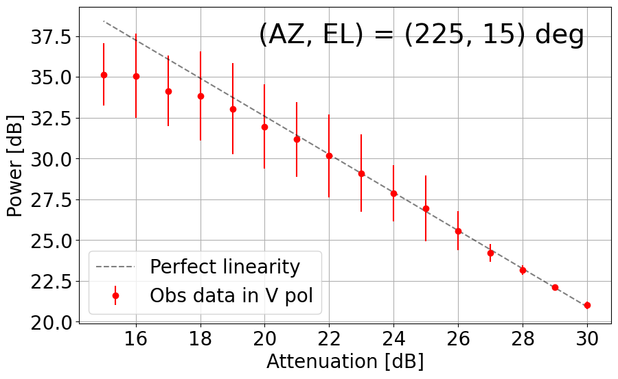
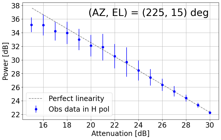

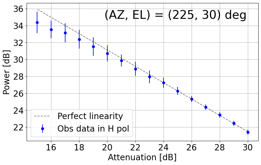

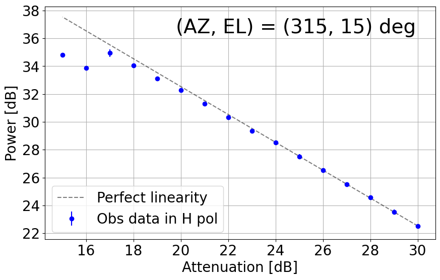
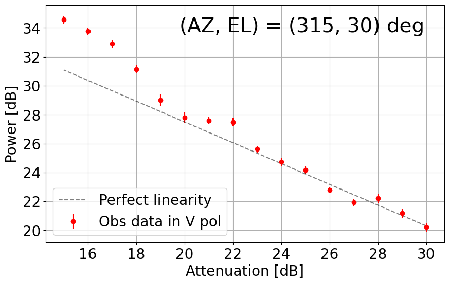
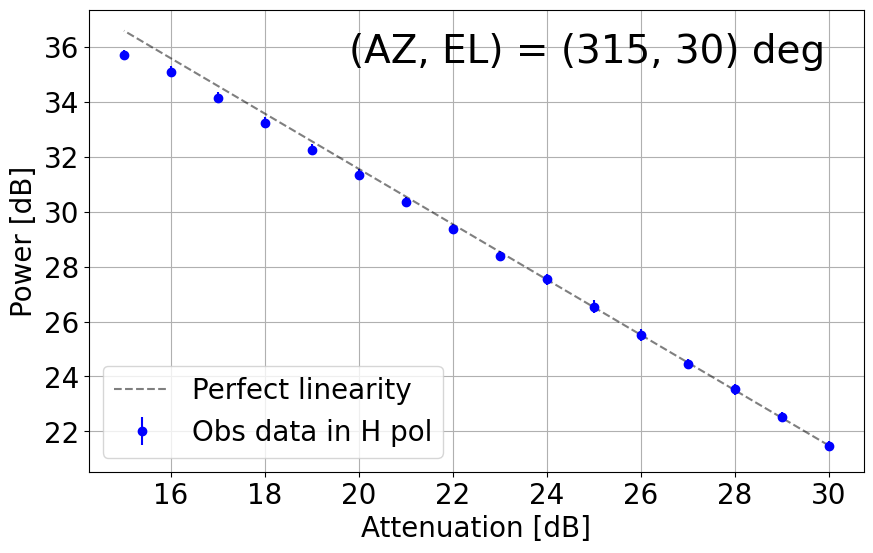
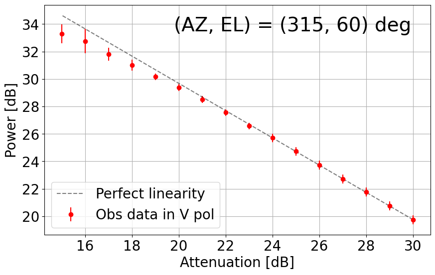
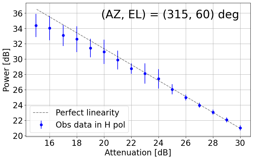
Figure 8-2: Results of linearity investigations in the current TNRT L-band system measured in the 1.417 - 1.423 GHz range for vertical (V, left) and horizontal (H, right) linear polarizations at (AZ, EL) = (45, 30), (135, 30), (225, 15), (225, 30), (315, 15), (315, 30) and (315, 60) deg. The rest of the caption is the same as in Figure 8-1.
9. Limitation of Integration Time at Each Observation Scanning
To verify a practical limitation of integration times at each observation scanning without an ON-OFF switching method on the nearby sky in the current TNRT L-band system, the relation between a standard deviation (1-sigma) of noise level and net integration time was investigated in Dec 2023 – Jan 2024 for dual linear polarization data. This investigation was completed at multiple positions of (AZ, EL) including the best transparent and the moderate Tsys* zones on the skyline maps, respectively. In these observations, each polarization data were obtained with 5-min scanning, and the frequency channel resolution was set to be 1.9 kHz that is proper for line emission observations in L-band. At post-processing stage, the data were analyzed in each different frequency range that is near the rest frequency of main/satellite OH masers (1612.231, 1665.402, 1667.359, and 1720.530 MHz) and 21-cm HI line emission (1420.40575 MHz) with 0.1 MHz integration, respectively.
As a result, improvement of 1-sigma rms noise level according to increment of integration times without ON-OFF switching in 0.1 MHz integration was achieved continuously according to theory at least within 5-min that was maximum in each observation scanning, for all the investigated frequency ranges and both dual linear polarizations, as shown in Figure 9-1.
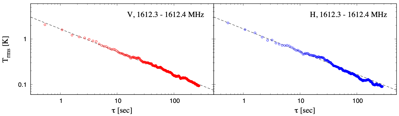
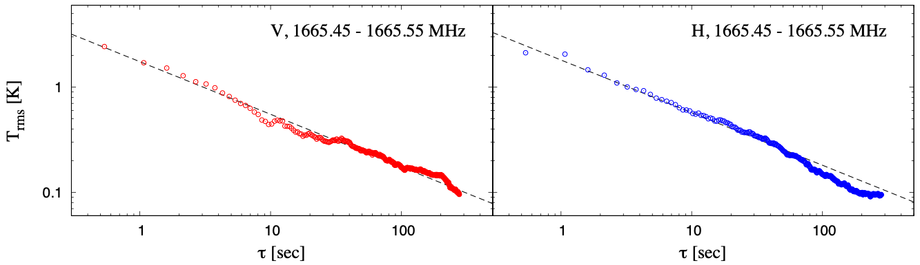
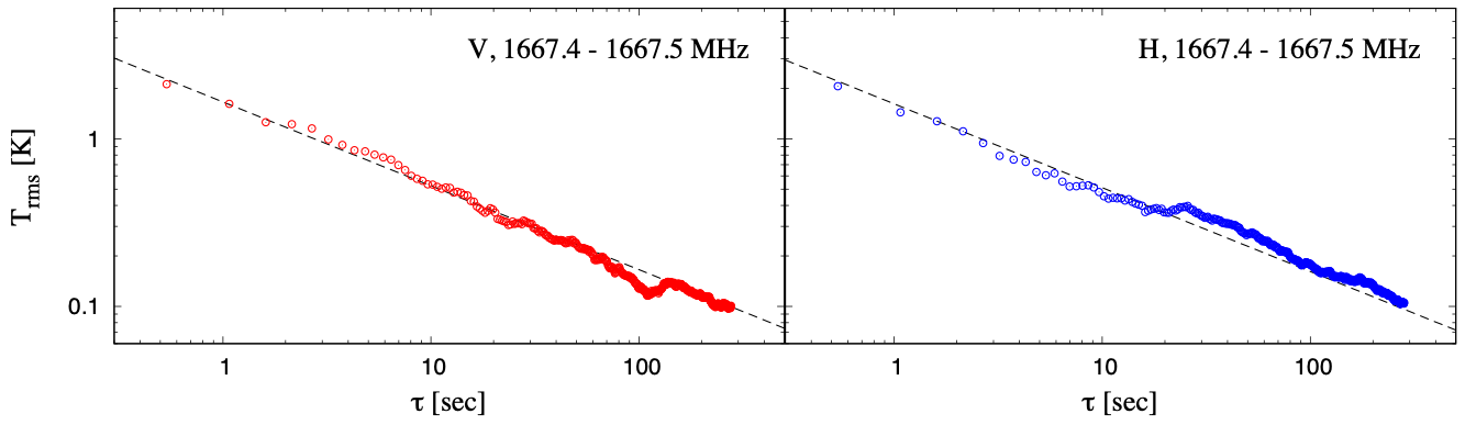

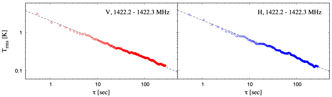
Figure 9-1: Relation between a standard deviation (1-sigma) of noise level and net integration time without ON-OFF switching method in the current TNRT L-band system measured for vertical (left-panels shown by red) and horizontal (right-panels shown by blue) linear polarizations, respectively, at (AZ, EL) = (315, 30) deg. Each panel from upper to lower shows the plots integrated by 0.1 MHz width in frequencies near main/satellite OH masers and 21-cm HI line emission rest frequencies, respectively. The vertical and horizontal axes correspond to 1-sigma rms noise level [K] and net integration time 𝜏 [sec]. The black dashed line in each panel shows the theoretical ideal case according to improvement by the inverse of square root of 𝜏.
The same verification but for guideline of net integration time without ON-OFF switching method for radio continuum emissions was also achieved at the same sky positions with the same observation set-up. At post-processing stage, the data were analyzed by integrating in the frequency range of 1660-1670 MHz, as shown in figure 9-2. Each plot for vertical (left-panel) and horizontal (right-panel) linear polarizations presented the limitation of achievable net integration time without ON-OFF switching up to approximately 2 min and 0.5 min, respectively. The difference of the possible net integration time between linear polarizations may be caused by RFI signals and its variability at the in-band.
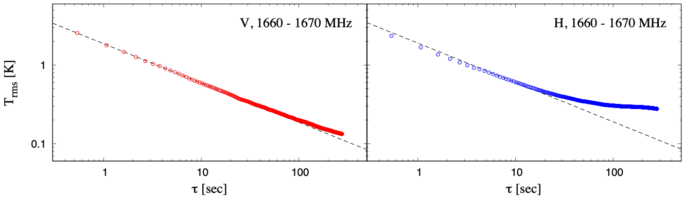
Figure 9-2: The same plots to figure 8-1 but for guideline of net integration time without ON-OFF switching method for radio continuum emissions measured for vertical (left-panels shown by red) and horizontal (right-panels shown by blue) linear polarizations, respectively, at (AZ, EL) = (315, 30) deg. Each panel shows the plots integrated by 10 MHz width in frequency range of 1660-1670 MHz.
Any Doppler tracking system in real time is not implemented in the current TNRT L-band system. The Doppler correction is thus performed at a post-processing calibration stage. This calibration works by calculating a velocity due to a Doppler effect at observatory, TNRO, on observing time corrected toward a target source direction in the Local Standard of Rest (LSR) frame with a developed python code.
Based on practical measured values of Tsys* = 15-30 K, a typical aperture efficiency 𝜂A of 50%, and the 8-bit sampling executed in the L-band receiver box for A/D conversion, the system equivalent flux density (SEFD) in the unit of Jansky of the current TNRT L-band system can be estimated by using the equation below:
SEFD = (2 k Tsys*)1026𝜂bit 𝜂A 𝝅D22
into be 66-132 Jy, where k is the Boltzmann constant, 𝜂bit is a coefficient to calibrate the quantization loss (≈ 1 in the case of 8-bit sampling), and D is the diameter of a telescope in the unit of meter.
As a result, RMS noise levels 𝜎rms in the case of observing with an integration time 𝝉 of 10 min for continuum and maser line emissions, respectively, can be typically calculated by using the equation below:
𝜎rms = SEFD×α(∆𝝂 𝝉)1/2
into be
Continuum case: 𝜎rms = 0.51 SEFD88 Jy100 MHz∆𝝂1/210 min𝝉1/2α21/2 mJy
Maser line case: 𝜎rms = 117 SEFD88 Jy1.9 kHz∆𝝂1/210 min𝝉1/2α21/2 mJy
where ∆𝝂 is a usable bandwidth assumed here to be 100 MHz and 1.9 kHz for continuum and maser emissions, respectively. The sensitivity decline factor α, depending on an observation method, is 2 if we apply the on-off position switching method for the baseline subtraction. We recommend applicants to fix the aforementioned usable bandwidth in your calculations. However, integration time is flexible depending on applicants' scientific requirements. Applicants are requested to consider a detection limit at least of 3 𝜎rms or higher to detect the target sources and to achieve applicants' scientific goals.
※ We note that the theoretical sensitivity is not achieved for TNRT observations of continuum sources, probably due to the rapid changes in the baseline. We recommend applicants to use the position (i.e., on-off) switching method with a short time interval where the target (continuum) source and the sky are observed alternately and quickly (e.g., < 30 sec).
We experimentally checked overhead time for TNRT observations. We repeated the 12-min (720 sec) observation by changing the single file integration time. (i.e., 20 sec * 36 files, 40 sec * 18 files,..., and 720 sec * 1 file). Note that the single-file integration time is divided evenly between on-source and off-source (i.e., sky) observations. Different frequency resolutions (100 and 2 kHz) were applied for continuum and spectral line observations, respectively.
Figure 12-1 shows that the overhead is inversely proportional to the integration time for a single file. In other words, the overhead is proportional to the number of files. If the integration time for a single file is 240 sec or longer, the overhead of spectral line observations is ~2-4 % larger than that of continuum observations. This is due to a larger file size for a spectral line observation.
We have a future plan to reduce the overhead by updating the back-end system of TNRT (i.e., software update). Considering the current overhead for TNRT observations (Figure 12-1), the stability of the TNRT L-band system (Figures 8-1 and 8-2), and single file size, we recommend a single file integration time of 120 sec (i.e., on-source = sky = 60 sec in a single file) or 180 sec for spectral line observations. That generates an overhead of 36 % or 24%. A 30% overhead is automatically included when the total request time for each proposal is calculated for a spectral line observation. Regarding the continuum observation, a single file integration time of 60 sec, corresponding to an overhead of ~70%, is applied.
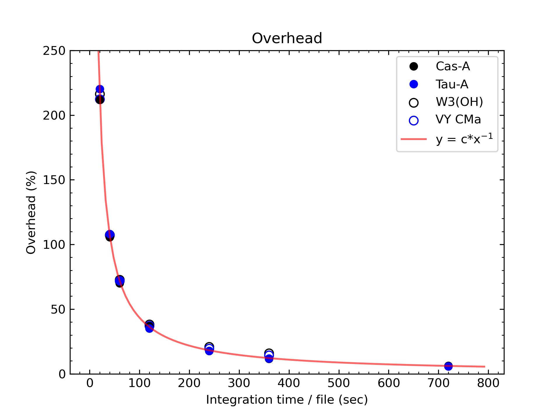
Figure 12-1: Experimental results for the overhead time of TNRT observations. A 12-min (720 sec) observation was repeated by changing the single-file integration time (i.e., 20 sec * 36 files, 40 sec * 18 files,..., and 720 sec * 1 file). Note that the single-file integration time is divided evenly between on-source and off-source (i.e., sky) observations. Different frequency resolutions, 100 and 2 kHz, were applied for continuum (filled symbols) and spectral line (open symbols) observations, respectively. Due to file size limitations, a single-file integration time of 720 sec could not be achieved for the spectral line observations. The data points are modeled by a power law function (red curve), y = 4218*x–0.997.
13. Observation Scanning Modes
In this CfP cycle, three observing scanning modes below are available:
[Single pointing] this mode is generally used for operations toward point (or point-like) target sources, unless other observing modes are requested.
[Cross scan] (e.g., figure 13-1 a) if applicants are concerned for less positional accuracies of the target source coordinates, this mode is recommended.
[Raster scan] (e.g., figure 13-1 b) this mode is recommended for a mapping observation toward diffuse target sources. The number of grids and a separation among each grid can be set flexibly. Typical overhead in the raster scan mode is around 30% of the total scanning time.
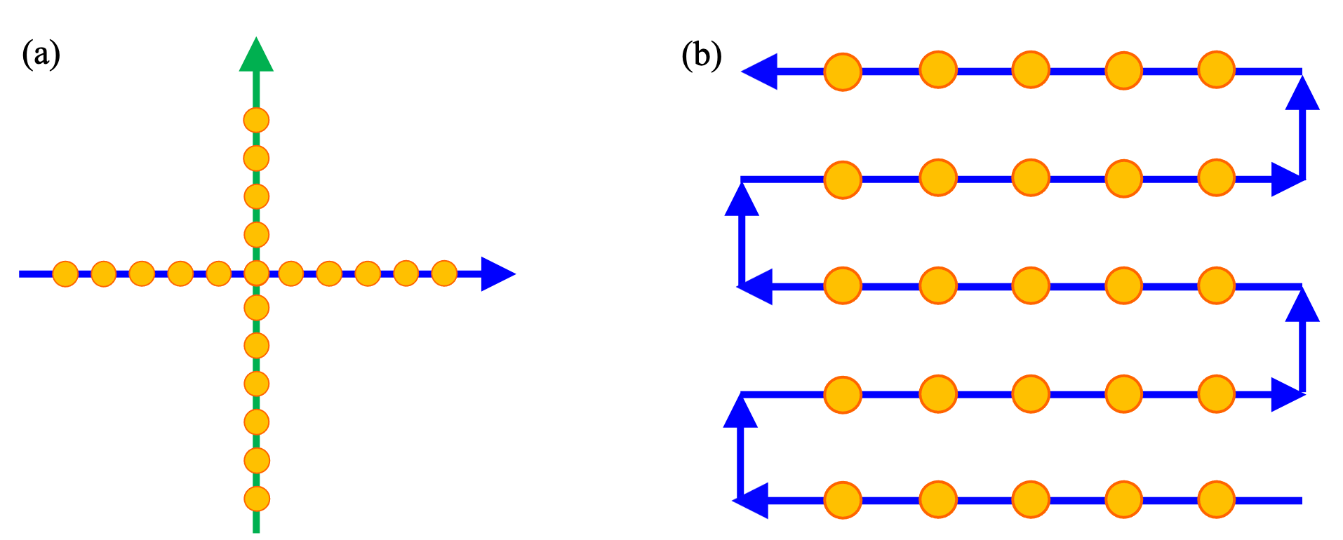
Figure 13-1: Schematic views of (a) cross scan mode, and (b) raster scan mode (an example in the case of 5 × 5 grid raster scan).
- de Vicente, P. & Barcia, A. 2007, Informe Técnio IT-OAN 2007-26
- Perley, R. A. & Butler, B. J. 2017, ApJS, 230, 7
- Ulich, B. L., & Haas, R. W. 1976, ApJS, 30, 247
- VLBA Calibrator Search Tool